Disclaimer:

1. Completely off-topic (please don't nuke this blog mike sir)
2. I don't know anything about statistics or how to judge the quality of a study.

There have been a couple of studies which have shown a statistically significant positive correlation between intelligence (measured through IQ) and physical attractiveness. The most popular one by number of citations is probably this. I will be referring to this study multiple times in this blog.

There are also a lot of studies which claim that perceived intelligence (what a random person would estimate your iq to be, by just looking at a photograph of your face) is positively correlated with measured intelligence (your actual iq), but they do not say anything about attractiveness (some examples are this and this).

Anyways, back to the first study I linked.

Now, why do I bring this up on codeforces of all places?

1. I love you guys and can't stop talking to you.
2. People here have a much higher average IQ than the general population, and yet everyone here seems to not have a girlfriend and repel women (maybe I'm projecting, but I see a lot of jokes about this in the comments and half of the userbase has an anime pfp. There also seems to be a joke that the lower your rating is, the less likely you are to be single.). Why isn't the average cf user a chad (or atleast chadlite) despite having big brain high iq genetics?

One could give a lot of reasons as to why this might be the case, with some truly big brain examples being:

1. Everyone here is a volcel, we could easily get females if we wanted but we're just too addicted to math/cp to seek females.
2. All the physically attractive smart males are too busy talking to females to do math, so only the less attractive smart males are congregating here.
3. Maybe only males in the 110-130 IQ range have good appearance genetics. Since we're all in the high 140s/low 150s, we have transcended humanity and do not have good look genes.
4. Most users here are actually chads but they refuse to reveal their chadness so other non-chad users don't feel bad about being looks mogged while IQ matched.

However, all the above reasons are bad and I couldn't think of any good reasons.

Therefore, to solve this mystery I decided to take advantage of my insanely high IQ and use the scientific method to explain this apparent contradiction. I request you, my brothers, in the name of science, to answer this extremely super scientific survey form to help me get to the bottom of this:

survey form

It is of course anonymous and I will publish the results (the primary focus being determining a positive or negative correlation between rating/iq and physical appearance) in a few days if the blogpost isn't nuked and enough people answer.

Hello codeforcers, since the editorial for 1930G - Prefix Max Set Counting is not out yet, and I found the problem to be pretty cute, I decided to write this blog.

Note:

1. I will refer to "prefix maximum array" as PMA for the sake of brevity.
2. By "possible" PMA, I mean a PMA which can be generated by some valid partial pre-order traversal.

Let us firstly make a couple of general observations:

1. If element $$$u$$$ occurs as a prefix maximum in any possible PMA, then the values of all its ancestors must be less than $$$u$$$.
2. If elements $$$i, j$$$ $$$(i < j)$$$ occur as adjacent prefix maximums in any possible PMA, then we have two cases:
   • $$$i$$$ is an ancestor of $$$j$$$ : Here, $$$i$$$ must be the largest (indexed) ancestor of $$$j$$$.
   • $$$i$$$ is not an ancestor of $$$j$$$: Here, let $$$c$$$ be the first node on the path from $$$lca(i, j)$$$ to $$$i$$$. $$$i$$$ must be the largest (indexed) node in the subtree of $$$c$$$ and $$$i$$$ must be larger (indexed) than the largest (indexed) ancestor of $$$j$$$.

Now, let's think about a slow solution, what if we were allowed to solve the problem in $$$O(n^2)$$$?

Well, a relatively simple idea that comes to mind is the following:

Define $$$dp_u$$$ to be the number of distinct PMA's we can get from a partial preorder traversal which ends at $$$u$$$, such that $$$u$$$ is the last element of the PMA.

Now, we try to compute all $$$dp_u$$$ in increasing order of $$$u$$$. Notice that the second last element $$$v$$$ in any PMA ending with $$$u$$$ must be $$$< u$$$, so to compute $$$dp_u$$$, we can iterate over every possible second last element $$$v$$$, and add the number of possible PMA's ending with $$$[v, u]$$$ to $$$dp_u$$$. It's important to fix the second last element to prevent overcounting (you will realise the motivating ideas later).

You now say, how do we find the number of such possible PMA's ending in $$$[v, u]$$$ for some given $$$u$$$ and $$$v$$$?

1. For there to exist any PMA ending with $$$[v, u]$$$, the conditions mentioned in observation $$$2$$$ must be satisfied by $$$v$$$ and $$$u$$$.
2. If the mentioned conditions are satisfied, then it can be shown that for every possible PMA ending with $$$v$$$ (call it $$$P$$$), it is possible to generate the PMA $$$P + [u]$$$. This is true because:
   • If $$$v$$$ is an ancestor of $$$u$$$: Simply go directly from $$$v$$$ to $$$u$$$ while performing the preorder traversal, and this will result in the PMA $$$P + [u]$$$.
   • If $$$v$$$ is not an ancestor of $$$u$$$: Perform the preorder traversal for the entire subtree of $$$c$$$ (same definition as in observation 2.b) and then go directly from $$$lca(u, v)$$$ to $$$u$$$. This results in the PMA $$$P + [u]$$$.

So, we now have a concrete $$$O(n^2)$$$ dp.

Optimizing this solution from $$$O(n^2)$$$ to $$$O(n\log{n})$$$ is honestly the easiest part of the problem and is a decent exercise as an implementation task on trees. I would advise you to try and do it yourself (there are several ways to do so).

I will just give a basic sketch of my (kinda ugly) implementation here. I won't go into as much detail as I did for describing the dp formulation because this blog is already way too long.

For any node $$$u$$$ (which doesn't trivially have $$$dp_u$$$ = 0), we make the following observations:

1. The only ancestor which contributes anything to $$$dp_u$$$ is the largest indexed ancestor (call it $$$mx$$$). (refer to observation 1 to see why this is true)
2. Other nodes which make a non-zero contribution to $$$dp_u$$$ are non-ancestral nodes.

   For any non-ancestral node $$$v$$$ which makes a non-zero contribution to $$$dp_u$$$, it's easy to see that $$$v$$$ must be the maximum node in the subtree of $$$c$$$ (first node on path from $$$lca(u, v)$$$ to $$$v$$$), Since $$$v < u$$$, this means that all nodes in the subtree of $$$c$$$ are smaller than $$$u$$$.

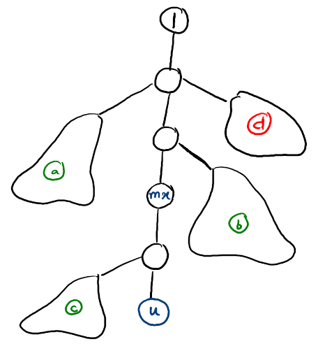
   Now, let's define a "blob node" (with respect to $$$u$$$): A blob node $$$x$$$ is a node such that all nodes in its subtree are less than $$$u$$$, and $$$u$$$ lies in the subtree of parent of $$$x$$$. We also define the representative of $$$x$$$, $$$rep_x$$$ to be the maximum indexed node in the subtree of $$$x$$$ (Clearly, $$$rep_x < u$$$).

   Claim : Any non-ancestral node $$$v$$$ ($$$< u$$$) which contributes something to $$$dp_u$$$ will be the representative of some blob node.
   Proof : Exercise for the reader, I am too tired.
   

   Let there be two sets of blobs : The set of Red blobs $$$R$$$ ($$$rep < mx$$$) and the set of Green blobs $$$G$$$ ($$$rep > mx$$$).

   This entire structure can be visualized in the following manner:

   ($$$mx$$$ is largest ancestor of $$$u$$$. $$$a$$$, $$$b$$$, $$$c$$$ are green blobs. $$$d$$$ is a red blob, it can be shown that parents of all red blobs are ancestors of $$$mx$$$).

   Clearly, $$$dp_u = dp_{mx} + [\sum{dp_{rep_x}} (x \in G)]$$$

   Which can be rewritten as $$$dp_u = dp_{mx} + [\sum{dp_{rep_x}} (x \in (R \cup G)] - [\sum{dp_{rep_x}} (x \in R)]$$$

   Now, how do we implement this?

   Maintaining blobs is pretty easy, you just have to keep pushing them upwards (see the remove() function in my code). For querying the second term for some $$$u$$$, we do the following: For any blob $$$x$$$ we will store $$$dp_{rep_x}$$$ at $$$par_x$$$ in some path sum query structure. Then, the second term is simply the sum on the path from the root node to $$$u$$$. Note that as the blob nodes move upwards/merge, you will have to make this change reflect in the path sum structure.

   As for the third term, this is a bit more tricky. It can be shown that the third term is actually equal to the (second term when $$$u = mx$$$), so for each node, we have to store the second term separately because it might be used later.

Surprisingly, the implementation isn't too cancerous: 247534020

Hello codeforcers, today I'll try to explain an alternate solution for this problem, which is completely different from any of the solutions mentioned in the editorial.

The solution works in $$$O((n + q)\sqrt{q} + q\log{q})$$$ time, and here is my shitty implementation with some comments.

Firstly, let us just find all the colors whose paths have the potential to be "good paths". Let's call these "potential paths". Clearly, each potential path will be a linear chain containing all the edges of its respective color. No two potential paths will share an edge (although they can share vertices). This can be easily done in $$$O(n)$$$ time.

Now, let's visualise a bipartite graph, between two sets of nodes: one set corresponding to colors (paths) and one set corresponding to vertices. An edge between color $$$c$$$ and vertex $$$v$$$ exists, if $$$v$$$ has an edge with color $$$c$$$. It's easy to show that this graph will have $$$2(n - 1)$$$ vertices at most (happens when each edge has a unique color).

If we were allowed to solve the problem in $$$O(qn)$$$ time, we could easily solve it using this graph and the following algorithm:

1. If we want to block/unblock vertex $$$p$$$, remove/restore all of the edges of its corresponding node in the bipartite graph.
2. The answer will be the weight of the maximum weighted potential path amongst all colors whose corresponding nodes do not have any deleted edges.

But this is obviously a dumb idea. What exactly is the problem here? The graph is too damn big, there are too many nodes and edges. So how do we remedy this? Well, obviously by making the graph smaller if possible.

Now, let's make an observation about how the bipartite graph is affected if we consider only a subset of all the vertices.

Observation: If we consider a set of $$$k$$$ vertices, there will be no more than $$$2(k - 1)$$$ "potential paths" which are touched by more than one vertex in this set.

Why is this true? Well, simply because the auxiliary tree of $$$k$$$ vertices has at most $$$2(k - 1)$$$ edges. Existence of more potential paths which are touched by more than one vertex from this set would imply that the auxiliary tree is incomplete which would be a contradiction.

Now, let us divide the queries into blocks of $$$\sqrt{q}$$$ size. We will be processing these blocks in order and answering queries.

At each block $$$B$$$, we will do the following:

Let $$$S$$$ be the set of nodes which will be toggled in $$$B$$$. Now, we can categorise all the "potential paths" into 3 types:

1. Type 1: Not touched by any node in $$$S$$$.
2. Type 2: Touched by exactly one node in $$$S$$$.
3. Type 3: Touched by $$$>1$$$ nodes in $$$S$$$.

This segregation can be done easily in $$$O(n)$$$ time.

There can be $$$O(n)$$$ type 1 and type 2 paths, but only $$$O(\sqrt{q})$$$ type 3 paths because of the observation we made above.

Let us see how we deal with each type:

1. Type 1: The validity of type 1 paths will not change throughout this block. So at the start of this block, we can easily compute in $$$O(n)$$$ time, that which of these paths are good. Let $$$mx$$$ be the weight of the maximum weight path among all the good type-1 potential paths.
2. Type 2: Even though there may be $$$O(n)$$$ such paths, we only really care about $$$O(\sqrt{q})$$$ of them. For each node $$$u$$$ in $$$S$$$, we only care about the maximum weight type-2 path that it touches, and the path has all its other nodes unblocked (so that, if $$$u$$$ is unblocked, this path becomes good). Throughout this block, we will now maintain a set which will contain weight of such path for each node in $$$S$$$ which is unblocked. Whenever we want to block/unblock some node, we can simply insert/erase its corresponding type-2 path's weight into the set.
3. Type 3: There are only $$$O(\sqrt{q})$$$ such paths, so we will simply use the slow solution I described above (just brute force updates and queries in the bipartite graph). Just construct the bipartite graph, it will have $$$O(\sqrt{q})$$$ nodes and $$$O(\sqrt{q})$$$ edges. Updates and queries both, will take $$$O(\sqrt{q})$$$ time.

So the answer for each query will simply be the maximum of the values we get from all the 3 types of paths, and time taken for each query will be $$$O(1 + \log{q} + \sqrt{q})$$$ (lol the holy trifecta).

Anyways, I hope there aren't any typos. I wrote this blog after eating 4 sizeable chocolates so I feel a bit disoriented. Good night. Harambe forever.