


Part 1: [Tutorial] My way of understanding Dinitz's ("Dinic's") algorithm
Part 2: [Tutorial] Minimum cost (maximum) flow
Part 3: [Tutorial] More about minimum cost flows: potentials and Dinitz
Introduction
There is a section in our ICPC notebook from 2019 called "min cost dinic". This blog started as an attempt to dissect what was written in there and understand why it works. In time, I needed to refer to many general ideas about flow, so it developed into a more general treatment of (min-cost) flow problems and spawned an entire separate blog about maximum flow and Dinitz. Even after splitting the blog, this blog was still too long, so I split it yet again. This blog will deal with the basic ideas of minimum cost flow; there will be a part 3, where I will generalize to a Dinitz-like algorithm and also talk a bit about something called potentials.
This blog is somewhat more technical and formal than I would ideally write, but there is a reason: there are things that one might overlook if they were not careful, and it is easy to gloss over something important. I remember well some misconceptions I used to have about flow back in the day. These algorithms are "fragile" — I don't mean that in a negative way, but they exist because a number of interesting facts come together, and being too informal may mean that we don't fully appreciate just how incredible it is.
Definition 1. Given a flow network $$$(G, c, s, t)$$$ and a cost function $$$a \colon\, E \to \mathbb{R}$$$ (in the following I will abbreviate this to "given a flow network $$$(G, c, a, s, t)$$$") the cost of a flow $$$f$$$ in $$$G$$$ is
The minimum cost maximum flow problem is to find a flow $$$f$$$ in $$$G$$$ such that the value of the flow is maximized, and among all possible solutions with maximum value, to find the one with minimum cost.
The aim of this blog is to prove the correctness of the "classical" minimum cost maximum flow algorithm (I have no idea if it has a name...):
Algorithm 2. Given a flow network $$$(G, c, a, s, t)$$$ without negative cycles.
- Initialize $$$f$$$ by setting $$$f(e) \gets 0$$$ for all edges.
- While $$$t$$$ is reachable from $$$s$$$ in $$$G_f$$$:
-
- Let $$$P$$$ be a shortest path from $$$s$$$ to $$$t$$$.
-
- Let $$$\gamma$$$ be the minimum capacity among the edges of $$$P$$$ in $$$G_f$$$.
-
- Define $$$\Delta f$$$ by putting $$$\gamma > 0$$$ flow on every edge in $$$P$$$.
-
- Let $$$f \gets f + \Delta f$$$.
- Return $$$f$$$.
Here and in the following, "shortest path" always means shortest with respect to edge costs (and not number of edges like in Edmonds-Karp).
Thanks to adamant and brunovsky for reviewing this blog. $$$~$$$
Basic theory of minimum cost flows
In this blog, we assume that the input network $$$(G, c, a, s, t)$$$ contains no negative cycles; that is, cycles whose sum of costs is negative.
It should be noted that the existence of negative cycles itself doesn't make minimum cost flow problems invalid, undefined or anything like that. Assuming all capacities are finite, it is not possible to end up with a "negative infinity" cost; it's just that negative cycles present a serious complication. There do however exist algorithms to deal with networks with negative cycles; I refer you to cycle-cancelling algorithms.
The reason why we work with no negative cycles in the initial network will be made clear in the course of the blog. There is quite a bit of discussion about negative cycles throughout. Most importantly, in the theory of min-cost flow, negative cycles are not some pathological case that we pretend doesn't exist (like it is for shortest paths), but rather, negative cycles are a quite central idea.
Also, simply negative costs do not present a problem. In fact, negative costs are incredibly useful in modeling problems with minimum cost flows.
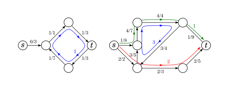
First, we must start by adapting the important concepts of maximum flow theory to the case of edge costs. The concept of a residual network remains much the same:
Definition 3. Given a flow network $$$(G, c, a, s, t)$$$ and a flow $$$f$$$, the residual flow network $$$G_f$$$ is a flow network defined as follows:
- The vertex set, source and sink vertices remain as they are.
- The edge set and its capacities and costs are defined like this. For each edge $$$e$$$ from $$$u$$$ to $$$v$$$:
-
- If $$$f(e) < c(e)$$$, $$$G_f$$$ has an edge $$$e$$$ from $$$u$$$ to $$$v$$$ with capacity $$$c_f(e) = c(e) - f(e)$$$ and cost $$$a_f(e) = a(e)$$$.
-
- If $$$0 < f(e)$$$, $$$G_f$$$ has an edge $$$\overleftarrow{e}$$$ from $$$v$$$ to $$$u$$$ with capacity $$$c_f(\overleftarrow{e}) = f(e)$$$ and cost $$$a_f(\overleftarrow{e}) = -a(e)$$$.
Pay attention to the fact that the reverse edges have costs with opposite sign compared to the original edges. This makes sense: putting flow on $$$\overleftarrow{e}$$$ represents removing flow from $$$e$$$, and if we do that, we want a refund on the cost we spent putting flow there.
Residual networks represent possible changes to flows the same way they did in the uncosted case.
Exercise 4. Given a flow network $$$(G, c, a, s, t)$$$, flows $$$f$$$, $$$f'$$$ on it $$$G$$$ and a flow $$$g$$$ on $$$G_f$$$. Show that:
- The flow $$$f' - f$$$ on $$$G_f$$$ has $$$\mathrm{cost}(f' - f) = \mathrm{cost}(f') - \mathrm{cost}(f)$$$.
- The flow $$$f + g$$$ on $$$G$$$ has $$$\mathrm{cost}(f + g) = \mathrm{cost}(f) + \mathrm{cost}(g)$$$.
- $$$(G_f)_g = G_{f + g}$$$ if we count parallel edges with the same cost as equal.
In several cases, it is convenient to refer to the decomposition of a flow into paths and cycles:
Theorem 5. Given a flow network $$$(G, c, s, t)$$$ (costs are unnecessary here) and a flow $$$f$$$. The flow $$$f$$$ can be "decomposed into paths and cycles": there exists a finite set $$$\mathcal{P}$$$ of paths from $$$s$$$ to $$$t$$$ and a finite set $$$\mathcal{C}$$$ of cycles. Each path $$$P$$$ and each cycle $$$C$$$ has a positive weight $$$w(P)$$$ ($$$w(C)$$$) such that
that is, the flow on each edge is the total weight of all paths and cycles that pass through it. In particular, if the value of the flow is 0 (such a flow is called a circulation), the path and cycle decomposition consists of just cycles.
Correctness of the classical algorithm
Recall the algorithm whose correctness we are trying to prove. I have made a small modification: for the moment, it is not important that $$$\gamma$$$ is the minimum capacity along the path. Since algorithm 2 is a special case of algorithm 6, proving the correctness of 6 also proves the correctness of 2.
Algorithm 6. Given a flow network $$$(G, c, a, s, t)$$$ without negative cycles.
- Initialize $$$f$$$ by setting $$$f(e) \gets 0$$$ for all edges.
- While $$$t$$$ is reachable from $$$s$$$ in $$$G_f$$$:
-
- Let $$$P$$$ be a shortest path from $$$s$$$ to $$$t$$$.
-
- Define $$$\Delta f$$$ by putting some $$$\gamma > 0$$$ flow on every edge in $$$P$$$.
-
- Let $$$f \gets f + \Delta f$$$.
- Return $$$f$$$.
Observation 7. Let $$$(G, c, a, s, t)$$$ be a flow network without negative cycles. Let $$$f$$$ be a flow on $$$G$$$ obtained by taking some shortest path $$$P$$$ from $$$s$$$ to $$$t$$$ and putting $$$\gamma$$$ flow on each edge of $$$P$$$. Then $$$G_f$$$ is without negative cycles.
This observation tells us that throughout the course of the algorithm, $$$G_f$$$ will not have any negative cycles, so we don't have to worry about negative cycles ever.
Note however, that this doesn't mean $$$G_f$$$ will not have any negative cycles for an arbitrary $$$f$$$! On the contrary, when we consider some $$$G_f$$$ and say that it doesn't have any negative cycles, care must be taken to make sure we actually have a basis for that claim. In fact,
Observation 8. Let $$$(G, c, a, s, t)$$$ be a flow network and $$$f$$$ a flow. $$$G_f$$$ has no negative cycles if and only if $$$f$$$ has minimum cost among all flows with value $$$\mathrm{val}(f)$$$.
Observations 7 and 8 put together elegantly show that all throughout the course of algorithm 6, the flow $$$f$$$ will always be the minimum cost flow for whatever value it is at right now. This proves the correctness of the algorithm. If it is minimum-cost for its value at every step, then it is certainly so at the end. Notice that algorithm 6 is a special case of the universal max-flow algorithm template (see part 1), whose correctness we already proved, so $$$f$$$ at the end must also be maximum. Finally, as long as we add a positive amount of flow at every step, which is certainly possible to, the algorithm terminates.
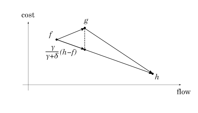
Minimum-cost flow as a piecewise linear function
There is an interesting corollary here. Notice that in algorithm 6, we never specified that the $$$\gamma$$$ must be the minimum capacity along the path $$$P$$$ (as is common in algorithms of Ford-Fulkerson type). It certainly can be, but we can pick $$$\gamma$$$ to be anything we want. Of course, it can't be more than the minimum capacity along $$$P$$$.
This means that at any given point in time, there is effectively a fixed cost --- the length of the shortest path — to transporting 1 unit of flow. We can take an arbitrarily small amount of flow, transport it with that cost, and it will be optimal. At some point the length of the shortest path changes and so will the cost. We have essentially proven that:
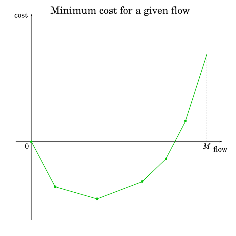
Corollary 9. Let $$$(G, c, a, s, t)$$$ be a flow network and $$$M$$$ the value of the maximum flow. The function
where $$$F(x)$$$ is defined as the minimum cost of a flow with value $$$x$$$, is piecewise linear.
Observation 10. The length of the shortest path in $$$G_f$$$ will never decrease throughout algorithm 6.
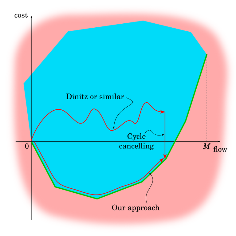
This means that $$$M(x)$$$ has a convex shape. At $$$x = 0$$$, $$$F(x) = 0$$$. As $$$x$$$ increases, $$$F(x)$$$ initially decreases, but gradually, its rate of decreasing decreases until eventually, it dips up again and starts increasing at an ever-faster rate. Of course, $$$F(x)$$$ may skip the decreasing part entirely and start increasing right away. Because of the piecewise linear nature of $$$F(x)$$$, these changes aren't smooth: the rate of change is constant, and then when the length of the shortest path changes, the rate of change abruptly increases.
Another way to see this is to recall the linear programming perspective of maximum flow. A flow can be seen as a point in $$$|E|$$$-dimensional space, where the $$$i$$$-th coordinate is the amount of flow on the $$$i$$$-th edge. The equalities and inequalities of the vertex and edge rules define the set of valid flows as a convex polytope. Project this polytope into two-dimensional space by mapping the value of the flow to the $$$x$$$-coordinate and the cost of the flow to the $$$y$$$-coordinate. Since these maps are linear, the projection is also a convex polytope, which means its lower boundary is a convex piecewise linear function.
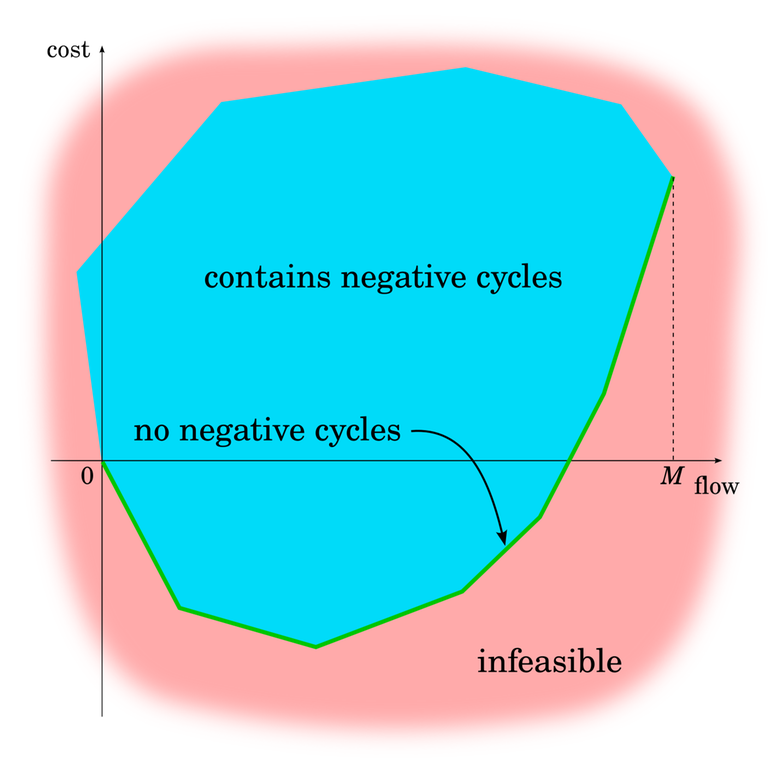
This is a good opportunity to talk a bit more about negative cycles. In this blog, we assumed that the input network doesn't have negative cycles and then proved that it keeps not having negative cycles. We see that our algorithm effectively moves along the green line at the bottom.
From the previous blog, we know that by just repeating steps of FF/EK/Dinitz, we can move left and right within the blue area, but can't control how much that moves us up and down.
Moving straight down in the blue area is also doable. I already mentioned cycle-cancelling algorithms and they are exactly it. Cycle-cancelling algorithms aren't anything particularly complex or difficult. It just means finding a negative cycle in $$$G_f$$$ and putting flow on each edge of it. If you pick the cycle with the minimum mean cost, it can be proven that this takes polynomial time, much like in Edmonds-Karp where you pick the path with the minimum cost.
This gives rise to another, different algorithm for minimum cost (maximum) flows, one that can actually handle negative cycles in the input. Use any maximum flow algorithm to calculate any flow ("move to the correct $$$x$$$-coordinate"), then use cycle-cancelling to go straight down.
Variations
I want to end this blog by discussing a couple of variations on the problem. Minimum cost maximum flow appears to be the most common variation in competitive programming; by contrast, university lectures and research literature seem most concerned with just minimum cost flow.
The machinery we have built here luckily allows us to easily switch between simple variants.
Minimum cost, fixed flow. In this problem, you are given the amount of flow and need to minimize the cost among such flows. Remember that we proved that at any stage of algorithm 2, the flow is minimum-cost and furthermore that minimum cost as a function of flow is piecewise linear.
The solution is therefore — if the flow we are about to push at some step of the algorithm would exceed the amount of flow we were told to achieve, only send through a fraction of the flow, then terminate the algorithm.
Minimum cost $$$b$$$-flow. In this problem, there is no source or sink. Instead, for each vertex $$$v$$$ we are given $$$b(v)$$$. Every vertex with $$$b(v) \ge 0$$$ is a "source" with exactly $$$b(v)$$$ flow coming in from "outside", and every vertex with $$$b(v) \le 0$$$ is a "sink" with exactly $$$b(v)$$$ flow leaving. You need to find the minimum cost flow that satisfies these constraints.
The solution is to reintroduce $$$s$$$ and $$$t$$$, which are sometimes called a "supersource" and a "supersink". Add an edge from $$$s$$$ to $$$v$$$ with capacity $$$b(v)$$$ and a cost $$$0$$$ for every $$$v$$$ with $$$b(v) \ge 0$$$, and do a similar thing with the supersink and the vertices with $$$b(v) \le 0$$$. Now we are in the "minimum cost, fixed flow" situation which we can already solve.
Minimum cost, any flow. In this problem, you need to find the minimum-cost flow among all valid flows. In principle, if sufficiently many edge costs are positive, this might just be the empty flow that doesn't send anything to anywhere. But presumably if you need to use this, you actually have some considerable negative edges.
The solution here is even simpler. The key is the convex nature of the minimum cost. All we need to do is to simply perform the algorithm as normal, and when the shortest path length becomes nonnegative, immediately terminate the algorithm.
Stay tuned for part 3!


Wow! Thank you for this, I've been looking for a good resource to learn this for a while!
Yet another epiq blog
Great post!
I've heard $$$b$$$-flow referred to as "circulation" for networks without costs, although I believe "Minimum cost circulation" typically means "Minimum cost, any flow". It feels like the literature on network problems has 100 names for each thing.
There's a nice trick that lets you go from edge lower bounds to $$$b$$$-flows; for an edge from $$$u \to v$$$ with lower bound $$$k$$$, add $$$k$$$ to the "sink-ness" of $$$u$$$ (subtract $$$k$$$ from $$$b(u)$$$), and add $$$k$$$ to the "source-ness" of $$$v$$$ (add $$$k$$$ to $$$b(v)$$$). Then each edge has capacity equal to its original capacity minus the lower bound. A solution to this $$$b$$$-flow is equivalent to a solution of the flow with lower bounds. This works with or without costs.
Then another variant is (min cost) max flow with edge lower bounds; find any solution to the lower bounds using the trick above, and then find a max flow on the residual graph. For networks without costs, you do this with two uses of a flow algorithm, but for networks with costs, I imagine you can do the first one that finds a lower bounds solution by using Dinitz, and then run your MCMF on the residual graph. Is there a better way to do this, perhaps even with only one use of a flow algorithm?
Find a lower bound solution with Dinitz or whatsoever, and cancel negative cycles which doesn't violate capacity constraints. Easiest way is to cancel minimum cost mean cycle, Hard way is to use Cost scaling MCMF. It can solve MCMF in $$$O(N^3 \log X)$$$ time :)
To say pedantically, "Circulation" and "Min Cost Circulation" is the only correct name to call them. If you think flows in a LP context, it is stupid to complicate things by introducing "source" and "sink". Why make two special cases that violate flow conservation? You can simply add an edge with infinite capacity from sink to source and compute a circulation.
Then, if you want "Minimum cost maximum flow", set the sink -> source edge's cost as $$$-\infty$$$ and compute Min cost circulation. If you want "Minimum cost any flow", set the cost $$$0$$$. If you want "Minimum cost fixed flow", set the lower and upper bound to desired value. That's why they don't deserve different names.
Auto comment: topic has been updated by -is-this-fft- (previous revision, new revision, compare).
Why exactly isn't it important? Isn't there a rule that $$$0 \le f(e)$$$. Because if you push $$$\gamma$$$ that is more than minimum on the path, there will be negative flow on an edge, which isn't allowed, won't there?