


[Part 1: [Tutorial] My way of understanding Dinitz's ("Dinic's") algorithm](104960) ↵
**Part 2: [Tutorial] Minimum cost (maximum) flow**↵
↵
#### Introduction↵
↵
There is a section in our ICPC notebook from 2019 called "min cost dinic".↵
This blog started as an attempt to dissect what was written in there and↵
understand why it works. In time, I needed to refer to many general ideas about↵
flow, so it developed into a more general treatment of (min-cost) flow problems↵
and spawned an entire separate blog about maximum flow and Dinitz. Even after↵
splitting the blog, this blog was still too long, so I split it yet again.↵
This blog will deal with the basic ideas of minimum cost flow; there will be a↵
part 3, where I will generalize to a Dinitz-like algorithm and also talk a bit↵
about something called potentials.↵
↵
This blog is somewhat more technical and formal than I would ideally write, but↵
there is a reason: there are things that one might overlook if they were not↵
careful, and it is easy to gloss over something important. I remember well↵
some misconceptions I used to have about flow back in the day. These algorithms↵
are "fragile" — I don't mean that in a negative way, but they exist because↵
a number of interesting facts come together, and being too informal may mean↵
that we don't fully appreciate just how incredible it is.↵
↵
**Definition 1.** Given a flow network $(G, c, s, t)$ and a _cost function_↵
$a \colon\, E \to \mathbb{R}$ (in the following I will abbreviate this to↵
"given a flow network $(G, c, a, s, t)$") the _cost_ of a flow $f$ in $G$ is↵
↵
$$ \mathrm{cost}(f) = \sum_{e \in E} f(e)ca(e). $$↵
↵
The _minimum cost maximum flow_ problem is to find a flow $f$ in $G$↵
such that the value of the flow is maximized, and among all possible↵
solutions with maximum value, to find the one with minimum cost.↵
↵
The aim of this blog is to prove the correctness of the "classical"↵
minimum cost maximum flow algorithm (I have no idea if it has a name...):↵
↵
**Algorithm 2.** Given a flow network $(G, c, a, s, t)$ without negative cycles.↵
↵
- Initialize $f$ by setting $f(e) \gets 0$ for all edges.↵
- While $t$ is reachable from $s$ in $G_f$:↵
- - Let $P$ be a shortest path from $s$ to $t$.↵
- - Let $\gamma$ be the minimum capacity among the edges of $P$ in $G_f$.↵
- - Define $\Delta f$ by putting $\gamma > 0$ flow on every edge in $P$.↵
- - Let $f \gets f + \Delta f$.↵
- Return $f$.↵
↵
Here and in the following, "shortest path" always means shortest with↵
respect to edge costs (and not number of edges like in Edmonds-Karp).↵
↵
Thanks to [user:adamant,2022-07-27] and [user:brunovsky,2022-07-27] for reviewing this blog.↵
↵
[cut] $~$↵
↵
#### Basic theory of minimum cost flows↵
↵
In this blog, we assume that the input network $(G, c, a, s, t)$↵
contains no negative cycles; that is, cycles whose sum of costs is↵
negative.↵
↵
It should be noted that the existence of negative cycles itself↵
doesn't make minimum cost flow problems invalid, undefined or anything↵
like that. Assuming all capacities are finite, it is not possible to↵
end up with a "negative infinity" cost; it's just that negative cycles↵
present a serious complication. There do however exist algorithms to↵
deal with networks with negative cycles; I refer you to cycle-cancelling↵
algorithms.↵
↵
The reason why we work with no negative cycles in the initial network↵
will be made clear in the course of the blog. There is quite a bit of↵
discussion about negative cycles throughout. Most importantly, in the theory↵
of min-cost flow, negative cycles are not some pathological case that ↵
we pretend doesn't exist (like it is for shortest paths), but rather,↵
negative cycles are a quite central idea.↵
↵
Also, simply negative costs do not present a problem. In fact,↵
negative costs are incredibly useful in modeling problems with minimum↵
cost flows. ↵
↵
First, we must start by adapting the important concepts of maximum↵
flow theory to the case of edge costs. The concept of a residual network↵
remains much the same:↵
↵
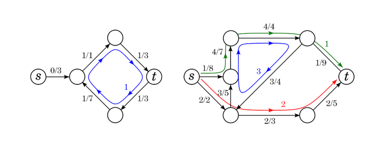
**Definition 3.** Given a flow network $(G, c, a, s, t)$ and a flow $f$,↵
the _residual flow network_ $G_f$ is a flow network defined as follows:↵
↵
- The vertex set, source and sink vertices remain as they are.↵
- The edge set and its capacities and costs are defined like this.↵
For each edge $e$ from $u$ to $v$:↵
- - If $f(e) < c(e)$, $G_f$ has an edge $e$ from $u$ to $v$↵
with capacity $c_f(e) = c(e) - f(e)$ and cost $a_f(e) = a(e)$.↵
- - If $0 < f(e)$, $G_f$ has an edge $\overleftarrow{e}$ from $v$ to $u$ with↵
capacity $c_f(\overleftarrow{e}) = f(e)$ and cost $a_f(\overleftarrow{e}) = -a(e)$.↵
↵
Pay attention to the fact that the reverse edges have costs with opposite sign↵
compared to the original edges. This makes sense: putting flow on $\overleftarrow{e}$↵
represents removing flow from $e$, and if we do that, we want a refund on the cost↵
we spent putting flow there.↵
↵
Residual networks represent possible changes to flows the same way↵
they did in the uncosted case.↵
↵
**Exercise 4.** Given a flow network $(G, c, a, s, t)$, flows $f$, $f'$ on it $G$ and↵
a flow $g$ on $G_f$. Show that:↵
↵
- The flow $f' - f$ on $G_f$ has $\mathrm{cost}(f' - f) = \mathrm{cost}(f') - \mathrm{cost}(f)$.↵
- The flow $f + g$ on $G$ has $\mathrm{cost}(f + g) = \mathrm{cost}(f) + \mathrm{cost}(g)$.↵
- $(G_f)_g = G_{f + g}$ if we count parallel edges with the same cost as equal.↵
↵
In several cases, it is convenient to refer to the decomposition of a flow↵
into paths and cycles:↵
↵
**Theorem 5.** Given a flow network $(G, c, s, t)$ (costs are unnecessary here)↵
and a flow $f$. The flow $f$ can be "decomposed into paths and cycles":↵
there exists a finite set $\mathcal{P}$ of paths from $s$ to $t$↵
and a finite set $\mathcal{C}$ of cycles. Each path $P$ and each cycle $C$↵
has a positive _weight_ $w(P)$ ($w(C)$) such that↵
↵
$$ f(e) = \displaystyle \sum_{P \in \mathcal{P}, e \in P} w(P) + \displaystyle \sum_{C \in \mathcal{C}, e \in C} w(C); $$↵
↵
that is, the flow on each edge is the total weight of all paths and cycles↵
that pass through it. In particular, if the value of the flow is 0 (such a ↵
flow is called a _circulation_), the path and cycle decomposition consists of just cycles.↵
↵
↵
↵
#### Correctness of the classical algorithm↵
↵
Recall the algorithm whose correctness we are trying to prove. I have made a small↵
modification: for the moment, it is not important that $\gamma$ is the minimum capacity↵
along the path. Since algorithm 2 is a special case of algorithm 6, proving the ↵
correctness of 6 also proves the correctness of 2.↵
↵
**Algorithm 6.** Given a flow network $(G, c, a, s, t)$ without negative cycles.↵
↵
- Initialize $f$ by setting $f(e) \gets 0$ for all edges.↵
- While $t$ is reachable from $s$ in $G_f$:↵
- - Let $P$ be a shortest path from $s$ to $t$.↵
- - Define $\Delta f$ by putting some $\gamma > 0$ flow on every edge in $P$.↵
- - Let $f \gets f + \Delta f$.↵
- Return $f$.↵
↵
**Observation 7.** Let $(G, c, a, s, t)$ be a flow network without negative↵
cycles. Let $f$ be a flow on $G$ obtained by taking some shortest path $P$↵
from $s$ to $t$ and putting $\gamma$ flow on each edge of $P$. Then↵
$G_f$ is without negative cycles.↵
↵
<spoiler summary="Proof">↵
Suppose that $G_f$ has a negative cycle $C$. Let $\delta$ be the↵
minimum capacity on $C$. Set $\epsilon = \min(\delta, \gamma)$ and consider↵
instead of $f$ the flow $f'$ obtained by putting $\epsilon$ flow on each↵
edge of $P$. Putting less flow can only add edges to the residual network,↵
so the conclusion will still be valid. Every edge in $C$ has capacity at↵
least $\epsilon$ in $G_{f'}$: edges of $G$ had their capacities increased↵
and reverse edges have a capacity of $\epsilon$.↵
↵
Define the flow $g$ on $G_{f'}$ by putting $\epsilon$ flow on each edge↵
of $C$. Clearly $\mathrm{cost}(g) < 0$. Consider the flow $f' + g = h$↵
on $G$. By the theorem above, we can decompose it to paths and cycles.↵
If we choose the path so that it has weight $\epsilon$, there will be↵
exactly one path. Either the cost of the path is less than the cost↵
of $P$, which is a contradiction with the assumption that $P$ is a shortest↵
path, or one of the cycles has negative cost, which is also a contradiction.↵
</spoiler>↵
↵
This observation tells us that throughout the course of the algorithm,↵
$G_f$ will not have any negative cycles, so we don't have to worry↵
about negative cycles ever.↵
↵
Note however, that this doesn't mean $G_f$ will not have any negative↵
cycles for an arbitrary $f$! On the contrary, when we consider some↵
$G_f$ and say that it doesn't have any negative cycles, care must be taken↵
to make sure we actually have a basis for that claim. In fact,↵
↵
**Observation 8.** Let $(G, c, a, s, t)$ be a flow network and $f$ a flow.↵
$G_f$ has no negative cycles if and only if $f$ has minimum cost among↵
all flows with value $\mathrm{val}(f)$.↵
↵
<spoiler summary="Proof">↵
Suppose that $f$ has minimum cost among all flows with value $\mathrm{val}(f)$.↵
If $G_f$ had a negative cycle, we could define a flow $g$ on $G_f$ by putting↵
some positive flow on each edge of the negative cycle. Then $\mathrm{val}(g) = 0$↵
but $\mathrm{cost}(g) < 0$, which means $\mathrm{val}(f) = \mathrm{val}(f + g)$↵
but $\mathrm{cost}(f + g) < \mathrm{cost}(f)$. Thus $G_f$ can not have negative↵
cycles.↵
↵
Suppose that $f$ does not have minimum cost among all flows with $\mathrm{val}(f)$↵
and there is some flow $f'$ with $\mathrm{val}(f) = \mathrm{val}(f')$ and↵
$\mathrm{cost}(f') < \mathrm{cost}(f)$. Then the value of $f' - f$ on $G_f$ is 0↵
and the cost of it is negative. The decomposition of $f' - f$ into paths↵
and cycles therefore consists of only cycles, and at least one of the cycles↵
must be negative.↵
</spoiler>↵
↵
Observations 7 and 8 put together elegantly show that all throughout the course↵
of algorithm 6, the flow $f$ will always be the minimum cost flow for whatever↵
value it is at right now. This proves the correctness of the algorithm. If↵
it is minimum-cost for its value at every step, then it is certainly so at↵
the end. Notice that algorithm 6 is a special case of the universal max-flow↵
algorithm template (see [part 1](104960)), whose correctness we already proved, so $f$ at the end↵
must also be maximum. Finally, as long as we add a positive amount of flow at every↵
step, which is certainly possible to, the algorithm terminates.↵
↵
#### Minimum-cost flow as a piecewise linear function↵
↵
There is an interesting corollary here. Notice that in algorithm 6, we never specified↵
that the $\gamma$ must be the minimum capacity along the path $P$ (as is common↵
in algorithms of Ford-Fulkerson type). It certainly can be, but we can pick $\gamma$↵
to be anything we want. Of course, it can't be more than the minimum capacity along $P$.↵
↵
This means that at any given point in time, there is effectively a fixed cost ---↵
the length of the shortest path — to transporting 1 unit of flow. We can take↵
an arbitrarily small amount of flow, transport it with that cost, and it will↵
be optimal. At some point the length of the shortest path changes and so will↵
the cost. We have essentially proven that:↵
↵
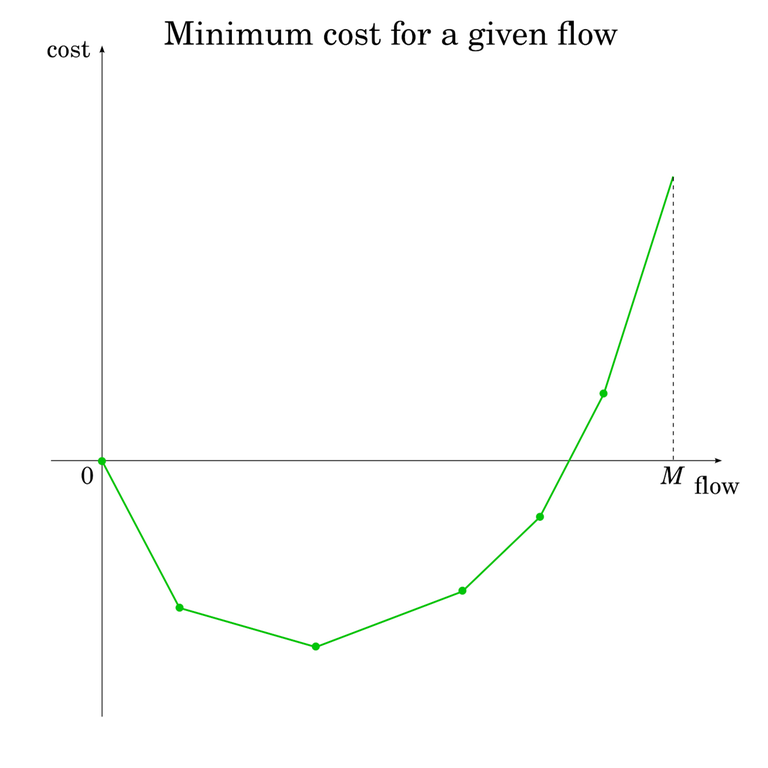
**Corollary 9.** Let $(G, c, a, s, t)$ be a flow network and $M$ the value of the↵
maximum flow. The function↵
↵
$$ F \colon\, [0, M] \to \mathbb{R}, $$↵
↵
where $F(x)$ is defined as the minimum cost of a flow with value $x$, is piecewise↵
linear.↵
↵
**Observation 10.** The length of the shortest path in $G_f$ will never decrease↵
throughout algorithm 6.↵
↵
<spoiler summary="Proof">↵
Suppose that $f, g, h$ are the flows at three successive states of algorithm 6.↵
That is,↵
↵
- We found some shortest path $P$ in $G_f$, added $\gamma > 0$ flow to each of them and got $g$.↵
- We found some shortest path $Q$ in $G_g$, added $\delta > 0$ flow to each of them and got $h$.↵
↵
If the cost of $Q$ was less than that of $P$, we could take the flow $h - f$ on $G_f$, rescale it so that it↵
has $\gamma$ flow and its cost would be smaller than the cost of $g$, contradicting the fact that↵
$g$ is minimum-cost.↵
↵
↵
↵
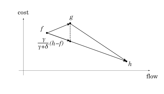
<spoiler summary="Ugly inequalities">↵
Since we add a positive amount of flow at each step, $\mathrm{val}(f) < \mathrm{val}(g) < \mathrm{val}(h)$.↵
Take the flow $h - f$ on $G_f$. Clearly↵
↵
$$ \mathrm{val}(h - f) = \gamma + \delta, \qquad \mathrm{cost}(h - f) = \gamma \, \mathrm{cost} (P) + \delta \, \mathrm{cost} (Q). $$↵
↵
Rescale the flow $h - f$ by $\frac{\gamma}{\gamma + \delta}$, that is, multiply↵
each edge's flow with that constant. Let the resulting flow be $k$. Then↵
$\mathrm{val}(k) = \mathrm{val}(g - f})$. We have already proven that $g$ has the minimum↵
cost for its value. Thus↵
↵
$$ \mathrm{cost}(k) = \frac{\gamma}{\gamma + \delta} (\gamma \, \mathrm{cost} (P) + \delta \, \mathrm{cost} (Q)) \ge \gamma \, \mathrm{cost} (P). $$↵
↵
Divide both sides by $\gamma$, rearrange and multiply out to get↵
↵
$$ \frac{\delta}{\gamma + \delta} \, \mathrm{cost} (Q) \ge \mathrm{cost} (P) - \frac{\gamma}{\gamma + \delta} \, \mathrm{cost} (P), $$↵
↵
which can be further rearranged and multiplied by $\frac{\gamma + \delta}{\delta}$ to obtain the desired inequality.↵
</spoiler>↵
↵
</spoiler>↵
↵
This means that $M(x)$ has a convex shape. At $x = 0$, $F(x) = 0$. As $x$ increases,↵
$F(x)$ initially decreases, but gradually, its rate of decreasing decreases↵
until eventually, it dips up again and starts increasing at an ever-faster rate.↵
Of course, $F(x)$ may skip the decreasing part entirely and start increasing↵
right away.↵
Because of the piecewise linear nature of $F(x)$, these changes aren't smooth:↵
the rate of change is constant, and then when the length of the shortest path↵
changes, the rate of change abruptly increases.↵
↵
↵
↵
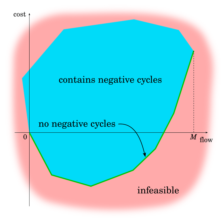
Another way to see this is to recall the linear programming perspective↵
of maximum flow. A flow can be seen as a point in $|E|$-dimensional space,↵
where the $i$-th coordinate is the amount of flow on the $i$-th edge.↵
The equalities and inequalities of the vertex and edge rules define↵
the set of valid flows as a convex polytope. Project this polytope into↵
two-dimensional space by mapping the value of the flow to the $x$-coordinate↵
and the cost of the flow to the $y$-coordinate. Since these maps are↵
linear, the projection is also a convex polytope, which means its lower boundary↵
is a convex piecewise linear function.↵
↵
↵
↵
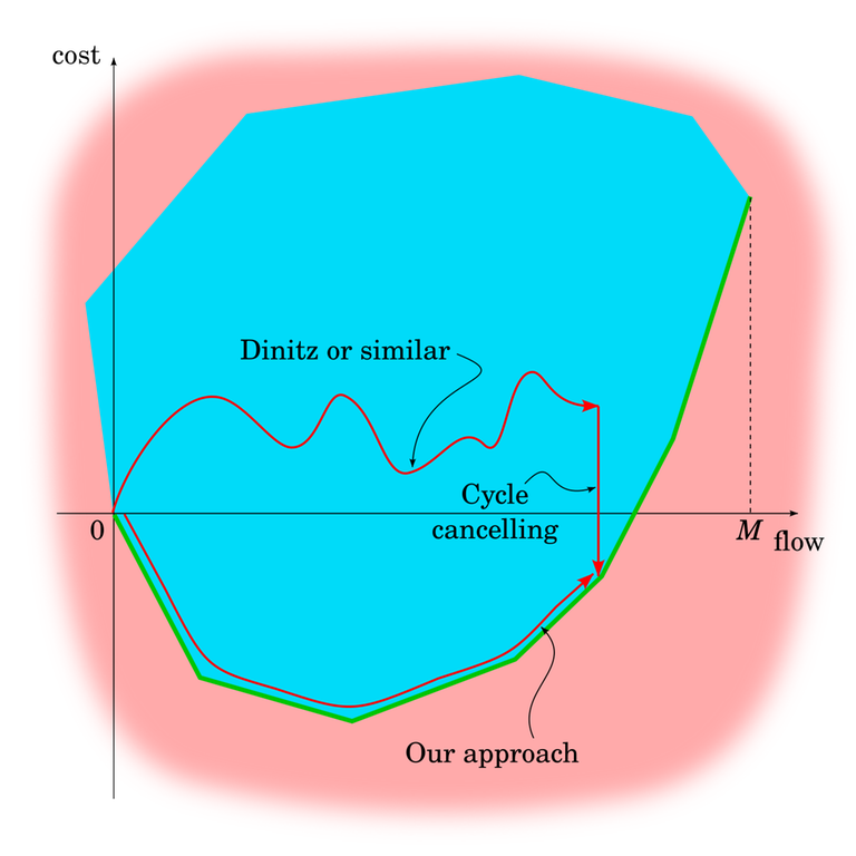
This is a good opportunity to talk a bit more about negative cycles. In this↵
blog, we assumed that the input network doesn't have negative cycles and↵
then proved that it keeps not having negative cycles. We see that our↵
algorithm effectively moves along the green line at the bottom.↵
↵
From the previous blog, we know that by just repeating steps of FF/EK/Dinitz,↵
we can move left and right within the blue area, but can't control how much↵
that moves us up and down.↵
↵
Moving straight down in the blue area is also doable. I already mentioned↵
cycle-cancelling algorithms and they are exactly it. Cycle-cancelling algorithms↵
aren't anything particularly complex or difficult. It just means finding a negative↵
cycle in $G_f$ and putting flow on each edge of it. If you pick the cycle with↵
the minimum mean cost, it can be proven that this takes polynomial time,↵
much like in Edmonds-Karp where you pick the path with the minimum cost.↵
↵
This gives rise to another, different algorithm for minimum cost (maximum)↵
flows, one that can actually handle negative cycles in the input.↵
Use any maximum flow algorithm to calculate any flow ("move to the correct $x$-coordinate"),↵
then use cycle-cancelling to go straight down.↵
↵
↵
↵
#### Variations↵
↵
I want to end this blog by discussing a couple of variations on the problem.↵
Minimum cost maximum flow appears to be the most common variation in competitive↵
programming; by contrast, university lectures and research literature seem most↵
concerned with just minimum cost flow.↵
↵
The machinery we have built here luckily allows us to easily switch between↵
simple variants. ↵
↵
**Minimum cost, fixed flow.** In this problem, you are given the amount of flow↵
and need to minimize the cost among such flows. Remember that we proved that↵
at any stage of algorithm 2, the flow is minimum-cost and furthermore that↵
minimum cost as a function of flow is piecewise linear.↵
↵
The solution is therefore — if the flow we are about to push at some step of↵
the algorithm would exceed the amount of flow we were told to achieve, only↵
send through a fraction of the flow, then terminate the algorithm.↵
↵
**Minimum cost $b$-flow.** In this problem, there is no source or sink. Instead,↵
for each vertex $v$ we are given $b(v)$. Every vertex with $b(v) \ge 0$ is a ↵
"source" with exactly $b(v)$ flow coming in from "outside", and every vertex with↵
$b(v) \le 0$ is a "sink" with exactly $b(v)$ flow leaving. You need to find ↵
the minimum cost flow that satisfies these constraints.↵
↵
The solution is to reintroduce $s$ and $t$, which are sometimes called a ↵
"supersource" and a "supersink". Add an edge from $s$ to $v$ with capacity $b(v)$↵
and a cost $0$ for every $v$ with $b(v) \ge 0$, and do a similar thing with the↵
supersink and the vertices with $b(v) \le 0$. Now we are in the "minimum cost,↵
fixed flow" situation which we can already solve.↵
↵
**Minimum cost, any flow.** In this problem, you need to find the minimum-cost↵
flow among all valid flows. In principle, if sufficiently many edge costs are↵
positive, this might just be the empty flow that doesn't send anything to anywhere.↵
But presumably if you need to use this, you actually have some considerable negative edges.↵
↵
The solution here is even simpler. The key is the convex nature of the minimum↵
cost. All we need to do is to simply perform the algorithm as normal, and when↵
the shortest path length becomes nonnegative, immediately terminate the algorithm.↵
↵
Stay tuned for part 3!
**Part 2: [Tutorial] Minimum cost (maximum) flow**↵
↵
#### Introduction↵
↵
There is a section in our ICPC notebook from 2019 called "min cost dinic".↵
This blog started as an attempt to dissect what was written in there and↵
understand why it works. In time, I needed to refer to many general ideas about↵
flow, so it developed into a more general treatment of (min-cost) flow problems↵
and spawned an entire separate blog about maximum flow and Dinitz. Even after↵
splitting the blog, this blog was still too long, so I split it yet again.↵
This blog will deal with the basic ideas of minimum cost flow; there will be a↵
part 3, where I will generalize to a Dinitz-like algorithm and also talk a bit↵
about something called potentials.↵
↵
This blog is somewhat more technical and formal than I would ideally write, but↵
there is a reason: there are things that one might overlook if they were not↵
careful, and it is easy to gloss over something important. I remember well↵
some misconceptions I used to have about flow back in the day. These algorithms↵
are "fragile" — I don't mean that in a negative way, but they exist because↵
a number of interesting facts come together, and being too informal may mean↵
that we don't fully appreciate just how incredible it is.↵
↵
**Definition 1.** Given a flow network $(G, c, s, t)$ and a _cost function_↵
$a \colon\, E \to \mathbb{R}$ (in the following I will abbreviate this to↵
"given a flow network $(G, c, a, s, t)$") the _cost_ of a flow $f$ in $G$ is↵
↵
$$ \mathrm{cost}(f) = \sum_{e \in E} f(e)
↵
The _minimum cost maximum flow_ problem is to find a flow $f$ in $G$↵
such that the value of the flow is maximized, and among all possible↵
solutions with maximum value, to find the one with minimum cost.↵
↵
The aim of this blog is to prove the correctness of the "classical"↵
minimum cost maximum flow algorithm (I have no idea if it has a name...):↵
↵
**Algorithm 2.** Given a flow network $(G, c, a, s, t)$ without negative cycles.↵
↵
- Initialize $f$ by setting $f(e) \gets 0$ for all edges.↵
- While $t$ is reachable from $s$ in $G_f$:↵
- - Let $P$ be a shortest path from $s$ to $t$.↵
- - Let $\gamma$ be the minimum capacity among the edges of $P$ in $G_f$.↵
- - Define $\Delta f$ by putting $\gamma > 0$ flow on every edge in $P$.↵
- - Let $f \gets f + \Delta f$.↵
- Return $f$.↵
↵
Here and in the following, "shortest path" always means shortest with↵
respect to edge costs (and not number of edges like in Edmonds-Karp).↵
↵
Thanks to [user:adamant,2022-07-27] and [user:brunovsky,2022-07-27] for reviewing this blog.↵
↵
[cut] $~$↵
↵
#### Basic theory of minimum cost flows↵
↵
In this blog, we assume that the input network $(G, c, a, s, t)$↵
contains no negative cycles; that is, cycles whose sum of costs is↵
negative.↵
↵
It should be noted that the existence of negative cycles itself↵
doesn't make minimum cost flow problems invalid, undefined or anything↵
like that. Assuming all capacities are finite, it is not possible to↵
end up with a "negative infinity" cost; it's just that negative cycles↵
present a serious complication. There do however exist algorithms to↵
deal with networks with negative cycles; I refer you to cycle-cancelling↵
algorithms.↵
↵
The reason why we work with no negative cycles in the initial network↵
will be made clear in the course of the blog. There is quite a bit of↵
discussion about negative cycles throughout. Most importantly, in the theory↵
of min-cost flow, negative cycles are not some pathological case that ↵
we pretend doesn't exist (like it is for shortest paths), but rather,↵
negative cycles are a quite central idea.↵
↵
Also, simply negative costs do not present a problem. In fact,↵
negative costs are incredibly useful in modeling problems with minimum↵
cost flows. ↵
↵
First, we must start by adapting the important concepts of maximum↵
flow theory to the case of edge costs. The concept of a residual network↵
remains much the same:↵
↵
**Definition 3.** Given a flow network $(G, c, a, s, t)$ and a flow $f$,↵
the _residual flow network_ $G_f$ is a flow network defined as follows:↵
↵
- The vertex set, source and sink vertices remain as they are.↵
- The edge set and its capacities and costs are defined like this.↵
For each edge $e$ from $u$ to $v$:↵
- - If $f(e) < c(e)$, $G_f$ has an edge $e$ from $u$ to $v$↵
with capacity $c_f(e) = c(e) - f(e)$ and cost $a_f(e) = a(e)$.↵
- - If $0 < f(e)$, $G_f$ has an edge $\overleftarrow{e}$ from $v$ to $u$ with↵
capacity $c_f(\overleftarrow{e}) = f(e)$ and cost $a_f(\overleftarrow{e}) = -a(e)$.↵
↵
Pay attention to the fact that the reverse edges have costs with opposite sign↵
compared to the original edges. This makes sense: putting flow on $\overleftarrow{e}$↵
represents removing flow from $e$, and if we do that, we want a refund on the cost↵
we spent putting flow there.↵
↵
Residual networks represent possible changes to flows the same way↵
they did in the uncosted case.↵
↵
**Exercise 4.** Given a flow network $(G, c, a, s, t)$, flows $f$, $f'$ on it $G$ and↵
a flow $g$ on $G_f$. Show that:↵
↵
- The flow $f' - f$ on $G_f$ has $\mathrm{cost}(f' - f) = \mathrm{cost}(f') - \mathrm{cost}(f)$.↵
- The flow $f + g$ on $G$ has $\mathrm{cost}(f + g) = \mathrm{cost}(f) + \mathrm{cost}(g)$.↵
- $(G_f)_g = G_{f + g}$ if we count parallel edges with the same cost as equal.↵
↵
In several cases, it is convenient to refer to the decomposition of a flow↵
into paths and cycles:↵
↵
**Theorem 5.** Given a flow network $(G, c, s, t)$ (costs are unnecessary here)↵
and a flow $f$. The flow $f$ can be "decomposed into paths and cycles":↵
there exists a finite set $\mathcal{P}$ of paths from $s$ to $t$↵
and a finite set $\mathcal{C}$ of cycles. Each path $P$ and each cycle $C$↵
has a positive _weight_ $w(P)$ ($w(C)$) such that↵
↵
$$ f(e) = \displaystyle \sum_{P \in \mathcal{P}, e \in P} w(P) + \displaystyle \sum_{C \in \mathcal{C}, e \in C} w(C); $$↵
↵
that is, the flow on each edge is the total weight of all paths and cycles↵
that pass through it. In particular, if the value of the flow is 0 (such a ↵
flow is called a _circulation_), the path and cycle decomposition consists of just cycles.↵
↵
↵
↵
#### Correctness of the classical algorithm↵
↵
Recall the algorithm whose correctness we are trying to prove. I have made a small↵
modification: for the moment, it is not important that $\gamma$ is the minimum capacity↵
along the path. Since algorithm 2 is a special case of algorithm 6, proving the ↵
correctness of 6 also proves the correctness of 2.↵
↵
**Algorithm 6.** Given a flow network $(G, c, a, s, t)$ without negative cycles.↵
↵
- Initialize $f$ by setting $f(e) \gets 0$ for all edges.↵
- While $t$ is reachable from $s$ in $G_f$:↵
- - Let $P$ be a shortest path from $s$ to $t$.↵
- - Define $\Delta f$ by putting some $\gamma > 0$ flow on every edge in $P$.↵
- - Let $f \gets f + \Delta f$.↵
- Return $f$.↵
↵
**Observation 7.** Let $(G, c, a, s, t)$ be a flow network without negative↵
cycles. Let $f$ be a flow on $G$ obtained by taking some shortest path $P$↵
from $s$ to $t$ and putting $\gamma$ flow on each edge of $P$. Then↵
$G_f$ is without negative cycles.↵
↵
<spoiler summary="Proof">↵
Suppose that $G_f$ has a negative cycle $C$. Let $\delta$ be the↵
minimum capacity on $C$. Set $\epsilon = \min(\delta, \gamma)$ and consider↵
instead of $f$ the flow $f'$ obtained by putting $\epsilon$ flow on each↵
edge of $P$. Putting less flow can only add edges to the residual network,↵
so the conclusion will still be valid. Every edge in $C$ has capacity at↵
least $\epsilon$ in $G_{f'}$: edges of $G$ had their capacities increased↵
and reverse edges have a capacity of $\epsilon$.↵
↵
Define the flow $g$ on $G_{f'}$ by putting $\epsilon$ flow on each edge↵
of $C$. Clearly $\mathrm{cost}(g) < 0$. Consider the flow $f' + g = h$↵
on $G$. By the theorem above, we can decompose it to paths and cycles.↵
If we choose the path so that it has weight $\epsilon$, there will be↵
exactly one path. Either the cost of the path is less than the cost↵
of $P$, which is a contradiction with the assumption that $P$ is a shortest↵
path, or one of the cycles has negative cost, which is also a contradiction.↵
</spoiler>↵
↵
This observation tells us that throughout the course of the algorithm,↵
$G_f$ will not have any negative cycles, so we don't have to worry↵
about negative cycles ever.↵
↵
Note however, that this doesn't mean $G_f$ will not have any negative↵
cycles for an arbitrary $f$! On the contrary, when we consider some↵
$G_f$ and say that it doesn't have any negative cycles, care must be taken↵
to make sure we actually have a basis for that claim. In fact,↵
↵
**Observation 8.** Let $(G, c, a, s, t)$ be a flow network and $f$ a flow.↵
$G_f$ has no negative cycles if and only if $f$ has minimum cost among↵
all flows with value $\mathrm{val}(f)$.↵
↵
<spoiler summary="Proof">↵
Suppose that $f$ has minimum cost among all flows with value $\mathrm{val}(f)$.↵
If $G_f$ had a negative cycle, we could define a flow $g$ on $G_f$ by putting↵
some positive flow on each edge of the negative cycle. Then $\mathrm{val}(g) = 0$↵
but $\mathrm{cost}(g) < 0$, which means $\mathrm{val}(f) = \mathrm{val}(f + g)$↵
but $\mathrm{cost}(f + g) < \mathrm{cost}(f)$. Thus $G_f$ can not have negative↵
cycles.↵
↵
Suppose that $f$ does not have minimum cost among all flows with $\mathrm{val}(f)$↵
and there is some flow $f'$ with $\mathrm{val}(f) = \mathrm{val}(f')$ and↵
$\mathrm{cost}(f') < \mathrm{cost}(f)$. Then the value of $f' - f$ on $G_f$ is 0↵
and the cost of it is negative. The decomposition of $f' - f$ into paths↵
and cycles therefore consists of only cycles, and at least one of the cycles↵
must be negative.↵
</spoiler>↵
↵
Observations 7 and 8 put together elegantly show that all throughout the course↵
of algorithm 6, the flow $f$ will always be the minimum cost flow for whatever↵
value it is at right now. This proves the correctness of the algorithm. If↵
it is minimum-cost for its value at every step, then it is certainly so at↵
the end. Notice that algorithm 6 is a special case of the universal max-flow↵
algorithm template (see [part 1](104960)), whose correctness we already proved, so $f$ at the end↵
must also be maximum. Finally, as long as we add a positive amount of flow at every↵
step, which is certainly possible to, the algorithm terminates.↵
↵
#### Minimum-cost flow as a piecewise linear function↵
↵
There is an interesting corollary here. Notice that in algorithm 6, we never specified↵
that the $\gamma$ must be the minimum capacity along the path $P$ (as is common↵
in algorithms of Ford-Fulkerson type). It certainly can be, but we can pick $\gamma$↵
to be anything we want. Of course, it can't be more than the minimum capacity along $P$.↵
↵
This means that at any given point in time, there is effectively a fixed cost ---↵
the length of the shortest path — to transporting 1 unit of flow. We can take↵
an arbitrarily small amount of flow, transport it with that cost, and it will↵
be optimal. At some point the length of the shortest path changes and so will↵
the cost. We have essentially proven that:↵
↵
**Corollary 9.** Let $(G, c, a, s, t)$ be a flow network and $M$ the value of the↵
maximum flow. The function↵
↵
$$ F \colon\, [0, M] \to \mathbb{R}, $$↵
↵
where $F(x)$ is defined as the minimum cost of a flow with value $x$, is piecewise↵
linear.↵
↵
**Observation 10.** The length of the shortest path in $G_f$ will never decrease↵
throughout algorithm 6.↵
↵
<spoiler summary="Proof">↵
Suppose that $f, g, h$ are the flows at three successive states of algorithm 6.↵
That is,↵
↵
- We found some shortest path $P$ in $G_f$, added $\gamma > 0$ flow to each of them and got $g$.↵
- We found some shortest path $Q$ in $G_g$, added $\delta > 0$ flow to each of them and got $h$.↵
↵
If the cost of $Q$ was less than that of $P$, we could take the flow $h - f$ on $G_f$, rescale it so that it↵
has $\gamma$ flow and its cost would be smaller than the cost of $g$, contradicting the fact that↵
$g$ is minimum-cost.↵
↵
↵
↵
<spoiler summary="Ugly inequalities">↵
Since we add a positive amount of flow at each step, $\mathrm{val}(f) < \mathrm{val}(g) < \mathrm{val}(h)$.↵
Take the flow $h - f$ on $G_f$. Clearly↵
↵
$$ \mathrm{val}(h - f) = \gamma + \delta, \qquad \mathrm{cost}(h - f) = \gamma \, \mathrm{cost} (P) + \delta \, \mathrm{cost} (Q). $$↵
↵
Rescale the flow $h - f$ by $\frac{\gamma}{\gamma + \delta}$, that is, multiply↵
each edge's flow with that constant. Let the resulting flow be $k$. Then↵
$\mathrm{val}(k) = \mathrm{val}(g - f
cost for its value. Thus↵
↵
$$ \mathrm{cost}(k) = \frac{\gamma}{\gamma + \delta} (\gamma \, \mathrm{cost} (P) + \delta \, \mathrm{cost} (Q)) \ge \gamma \, \mathrm{cost} (P). $$↵
↵
Divide both sides by $\gamma$, rearrange and multiply out to get↵
↵
$$ \frac{\delta}{\gamma + \delta} \, \mathrm{cost} (Q) \ge \mathrm{cost} (P) - \frac{\gamma}{\gamma + \delta} \, \mathrm{cost} (P), $$↵
↵
which can be further rearranged and multiplied by $\frac{\gamma + \delta}{\delta}$ to obtain the desired inequality.↵
</spoiler>↵
↵
</spoiler>↵
↵
This means that $M(x)$ has a convex shape. At $x = 0$, $F(x) = 0$. As $x$ increases,↵
$F(x)$ initially decreases, but gradually, its rate of decreasing decreases↵
until eventually, it dips up again and starts increasing at an ever-faster rate.↵
Of course, $F(x)$ may skip the decreasing part entirely and start increasing↵
right away.↵
Because of the piecewise linear nature of $F(x)$, these changes aren't smooth:↵
the rate of change is constant, and then when the length of the shortest path↵
changes, the rate of change abruptly increases.↵
↵
↵
↵
Another way to see this is to recall the linear programming perspective↵
of maximum flow. A flow can be seen as a point in $|E|$-dimensional space,↵
where the $i$-th coordinate is the amount of flow on the $i$-th edge.↵
The equalities and inequalities of the vertex and edge rules define↵
the set of valid flows as a convex polytope. Project this polytope into↵
two-dimensional space by mapping the value of the flow to the $x$-coordinate↵
and the cost of the flow to the $y$-coordinate. Since these maps are↵
linear, the projection is also a convex polytope, which means its lower boundary↵
is a convex piecewise linear function.↵
↵
↵
↵
This is a good opportunity to talk a bit more about negative cycles. In this↵
blog, we assumed that the input network doesn't have negative cycles and↵
then proved that it keeps not having negative cycles. We see that our↵
algorithm effectively moves along the green line at the bottom.↵
↵
From the previous blog, we know that by just repeating steps of FF/EK/Dinitz,↵
we can move left and right within the blue area, but can't control how much↵
that moves us up and down.↵
↵
Moving straight down in the blue area is also doable. I already mentioned↵
cycle-cancelling algorithms and they are exactly it. Cycle-cancelling algorithms↵
aren't anything particularly complex or difficult. It just means finding a negative↵
cycle in $G_f$ and putting flow on each edge of it. If you pick the cycle with↵
the minimum mean cost, it can be proven that this takes polynomial time,↵
much like in Edmonds-Karp where you pick the path with the minimum cost.↵
↵
This gives rise to another, different algorithm for minimum cost (maximum)↵
flows, one that can actually handle negative cycles in the input.↵
Use any maximum flow algorithm to calculate any flow ("move to the correct $x$-coordinate"),↵
then use cycle-cancelling to go straight down.↵
↵
↵
↵
#### Variations↵
↵
I want to end this blog by discussing a couple of variations on the problem.↵
Minimum cost maximum flow appears to be the most common variation in competitive↵
programming; by contrast, university lectures and research literature seem most↵
concerned with just minimum cost flow.↵
↵
The machinery we have built here luckily allows us to easily switch between↵
simple variants. ↵
↵
**Minimum cost, fixed flow.** In this problem, you are given the amount of flow↵
and need to minimize the cost among such flows. Remember that we proved that↵
at any stage of algorithm 2, the flow is minimum-cost and furthermore that↵
minimum cost as a function of flow is piecewise linear.↵
↵
The solution is therefore — if the flow we are about to push at some step of↵
the algorithm would exceed the amount of flow we were told to achieve, only↵
send through a fraction of the flow, then terminate the algorithm.↵
↵
**Minimum cost $b$-flow.** In this problem, there is no source or sink. Instead,↵
for each vertex $v$ we are given $b(v)$. Every vertex with $b(v) \ge 0$ is a ↵
"source" with exactly $b(v)$ flow coming in from "outside", and every vertex with↵
$b(v) \le 0$ is a "sink" with exactly $b(v)$ flow leaving. You need to find ↵
the minimum cost flow that satisfies these constraints.↵
↵
The solution is to reintroduce $s$ and $t$, which are sometimes called a ↵
"supersource" and a "supersink". Add an edge from $s$ to $v$ with capacity $b(v)$↵
and a cost $0$ for every $v$ with $b(v) \ge 0$, and do a similar thing with the↵
supersink and the vertices with $b(v) \le 0$. Now we are in the "minimum cost,↵
fixed flow" situation which we can already solve.↵
↵
**Minimum cost, any flow.** In this problem, you need to find the minimum-cost↵
flow among all valid flows. In principle, if sufficiently many edge costs are↵
positive, this might just be the empty flow that doesn't send anything to anywhere.↵
But presumably if you need to use this, you actually have some considerable negative edges.↵
↵
The solution here is even simpler. The key is the convex nature of the minimum↵
cost. All we need to do is to simply perform the algorithm as normal, and when↵
the shortest path length becomes nonnegative, immediately terminate the algorithm.↵
↵
Stay tuned for part 3!

