


Hello everybody,
I've built a function that can be used to display a graph using GraphViz's dot tool. You need to have the dot tool installed or you can copy the graph.dot file to an online dot viewer.
On Ubuntu, this can be installed with the following command: sudo apt install dot
The command works on Linux but will need to be changed on other OSes like Windows. You can copy this function and use it while debugging graph problems.
#include <bits/stdc++.h>
using namespace std;
void show_graph(const vector<vector<int>> &graph, const bool undirected = true) {
/*! Converts graph to dot format
*\param undirected is whether graph is undirected or not */
ofstream os{"graph.dot"};
os << (undirected ? "graph" : "digraph");
os << " G {" << endl;
for(int u = 0; u < graph.size(); ++u) {
for (const auto v : graph[u]) {
if (!undirected || u <= v) {
os << "\t" << u << (undirected ? " -- " : " -> ") << v << endl;
}
}
}
os << "}" << endl;
/* Displays dot using image viewer
/ This command is for Linux. You can change this command for a different OS or for a different image viewer.*/
system("dot -Tpng graph.dot -o graph.png && xdg-open graph.png");
}
void add_edge(vector<vector<int>>& graph, const int u, const int v){
/*! Add edge (u, v) to graph*/
graph[u].push_back(v);
graph[v].push_back(u);
}
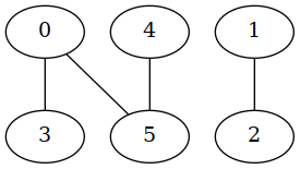
int main(){
vector<vector<int>> graph(6);
add_edge(graph, 1, 2);
add_edge(graph, 0, 3);
add_edge(graph, 4, 5);
add_edge(graph, 0, 5);
show_graph(graph, true);
}
Dot file produced (graph.dot):
graph G {
        0 -- 3
        0 -- 5
        1 -- 2
        4 -- 5
}
The image produced (graph.png):
You can find other useful utilities like this in my template library.


