Introduction
There are a number of "small" algorithms and facts that come up again and again in problems. I feel like there I have had to explain them many times, partly because there are no blogs about them. On the other hand, writing a blog about them is also weird because there is not that much to be said. To settle these things "once and for all", I decided to write my own list about about common "small tricks" that don't really warrant a full tutorial because they can be adequately explained in a paragraph or two and there often isn't really anything to add except for padding.
This blog is partly inspired by adamant's blog from a few years ago. At first, I wanted to mimic adamant's blog structure exactly, but I found myself wanting to write longer paragraphs and using just bolded sentences as section headers got messy. Still, each section is short enough that it would not make much sense to write separate blogs about each of these things.
All of this is well-known to some people, I don't claim ownership or novelty of any idea here.
1. Memory optimization of bitset solutions
In particular, reachable nodes in a DAG. Consider the following problem. Given a DAG with $$$n$$$ vertices and $$$m$$$ edges, you are given $$$q$$$ queries of the form "is the vertex $$$v$$$ reachable from the vertex $$$u$$$". $$$n, m, q \le 10^5$$$. The memory limit does not allow $$$O(n^2)$$$ or similar space complexity. This includes making $$$n$$$ bitsets of length $$$n$$$.
A classical bitset solution is to let $$$\mathrm{dp}[v]$$$ be a bitset such that $$$\mathrm{dp}[v][u] = 1$$$ iff $$$v$$$ is reachable from $$$u$$$. Then $$$\mathrm{dp}[v]$$$ can be calculated simply by taking the bitwise or of all its immediate predecessors and then setting the $$$v$$$-th bit to 1. This solution almost works, but storing $$$10^5$$$ bitsets of size $$$10^5$$$ takes too much memory in most cases. To get around this, we use 64-bit integers instead of bitsets and repeat this procedure $$$\frac{n}{64}$$$ times. In the $$$k$$$-th phase of this algorithm, we let $$$\mathrm{dp}[v]$$$ be a 64-bit integer that stores whether $$$v$$$ is reachable from the vertices $$$64k, 64k + 1, \ldots, 64k + 63$$$.
In certain circles, this problem has achieved a strange meme status. Partly, I think it is due to how understanding of the problem develops. At first, you don't know how to solve the problem. Then, you solve it with bitsets. Then, you realize it doesn't work and finally you learn how to really solve it. Also, it is common to see someone asking how to solve this, then someone else will always reply something along the lines of "oh, you foolish person, don't you realize it is just bitsets?" and then you get to tell them that they're also wrong.
Besides the classical reachability problem, I also solved AGC 041 E this way.
2. Avoiding logs in Mo's algorithm
Consider the following problem. Given an array $$$A$$$ of length $$$n$$$ and $$$n$$$ queries of the form "given $$$l$$$ and $$$r$$$, find the MEX of $$$A[l], \ldots, A[r]$$$". Queries are offline, i.e. all queries are given in the input at the beginning, it is not necessary to answer a query before reading the next one. $$$n \le 10^5$$$.
The problem can also be solved with segment trees avoiding a square-root factor altogether. In this blog however, we consider Mo's algorithm. Don't worry, this idea can be applied in many situations and a segment tree solution might not always be possible.
A first attempt at solving might go like this. As always, we maintain an active segment. We keep a set<int> of all integers up to $$$n$$$ that are not represented in the active segment, and an auxiliary array to count how many times each number appears in the active segment. In $$$O(\log n)$$$ time we can move an endpoint of the active segment, and in $$$O(\log n)$$$ time we can find the MEX of the active segment. We move the endpoints one by one to go through all queries, and if the queries are sorted in a certain magical order, we get $$$O(n \sqrt n \log n)$$$ complexity. Unfortunately, this is too slow; also $$$O(n \sqrt n \log n)$$$ is an altogether evil complexity and should be avoided at all costs.
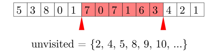
Clearly, set<int> is a bottleneck. Why do we use it? We need to support the following operations on a set:
- Insert an element. Currently $$$O(\log n)$$$. Called $$$O(n \sqrt n)$$$ times.
- Remove an element. Currently $$$O(\log n)$$$. Called $$$O(n \sqrt n)$$$ times.
- Find the minimum element. Currently $$$O(\log n)$$$. Called $$$O(n)$$$ times.
Note that operations 1 and 2 are more frequent than 3, but they take the same amount of time. To optimize, we should "balance" this: we need 1 and 2 to be faster, but it's fine if this comes at the expense of a slightly slower operation 3. What we need is a data structure that does the following:
- Insert an element in $$$O(1)$$$.
- Delete an element in $$$O(1)$$$.
- Find the minimum element in $$$O(\sqrt n)$$$.
Description of the data structureThe set only needs to contain elements from the range $$$0, \ldots, n$$$. We maintain an array telling us whether each element is in the set. Now, we divide the array into blocks of length $$$\sqrt n$$$. For each block, we maintain the number of elements present in the set in this block. Inserting and deleting an element can be done in $$$O(1)$$$ time — update the array and the block. To find the minimum element, we iterate over the blocks to find the first one that isn't empty, then iterate over the elements of that block to find the minimum one that's present. The time complexity of doing that in $$$O(\sqrt n)$$$.
This should be treated as the main part of the trick: to make sure endpoints can be moved in $$$O(1)$$$ time, potentially at the expense of query time. How the data structure actually works is actually even not that important; in a different problem, this data structure might be something different.
3. Square root optimization of knapsack/"$$$3k$$$ trick"
Assume you have $$$n$$$ rocks with nonnegative integer weights $$$a_1, a_2, \ldots, a_n$$$ such that $$$a_1+a_2+\cdots+a_n = m$$$. You want to find out if there is a way to choose some rocks such that their total weight is $$$w$$$.
Suppose there are three rocks with equal weights $$$a, a, a$$$. Notice that it doesn't make any difference if we replace these three rocks with two rocks with weights $$$a, 2a$$$. We can repeat this process of replacing until there are at most two rocks of each weight. The sum of weights is still $$$m$$$, so there can be only $$$O(\sqrt m)$$$ rocks (see next point). Now you can use a classical DP algorithm but with only $$$O(\sqrt m)$$$ elements, which can be lead to a better complexity in many cases.
This trick mostly comes up when the $$$a_1, a_2, \ldots, a_n$$$ form a partition of some kind. For example, maybe they represent connected components of a graph. See the example.
Worked example: KeyboardThis problem is from Baltic Olympiad in Informatics 2021, practice round. Link to the problem.
You are given a dictionary of $$$m$$$ different words over an alphabet of $$$n$$$ letters. You want to color the letters in two colors such that in every word the letters alternate between the colors (the problem statement mentions building an ergonomic keyboard with a "left" half and a "right" half). Minimize the difference between the number of red letters and the number of blue letters.
The idea is to view the whole thing as a bipartite graph. The input generates some number of connected components and we can "flip" some of the components to make the sides as equal as possible. Initially, flip all the components so that the left side is smaller. Now we have to flip some components again: for the $$$i$$$-th component, flipping it would increase the size of the left half by some $$$a_i$$$, and we have to choose some of the components to flip such that their sum is as close to a certain integer as possible. Since $$$\sum a_i \le n$$$, we can use this trick to solve the problem in time $$$O(n \sqrt n)$$$.
I believe that to get full points, you have to combine this with bitsets.
4. Number of unique elements in a partition
This is also adamant's number 13, but I decided to repeat it because it ties into the previous point. Assume there are $$$n$$$ nonnegative integers $$$a_1, a_2, \ldots, a_n$$$ such that $$$a_1 + a_2 + \cdots + a_n = m$$$. Then there are only $$$O(\sqrt m)$$$ distinct values among $$$a_1, a_2, \ldots, a_n$$$.
ProofTake out the distinct values, sort them, let them be $$$b_0, b_1, \ldots, b_{k - 1}$$$. Because the values $$$b_i$$$ are nonnegative sorted integers, we must have $$$b_i \ge i$$$. Therefore
$$$b_0 + b_1 + \cdots + b_{k - 1} \ge 0 + 1 + \cdots + (k - 1) = \frac{k(k - 1)}{2}.$$$On the other hand, $$$b_0 + b_1 + \cdots + b_{k - 1} \le m$$$, so we obtain $$$\frac{k(k - 1)}{2} \le m$$$. Now it is easy to see that $$$k$$$ is $$$O(\sqrt{m})$$$.
5. Removing elements from a knapsack
Suppose there are $$$n$$$ rocks, each with a weight $$$w_i$$$. You are maintaining an array $$$\mathrm{dp}[i]$$$, where $$$\mathrm{dp}[i]$$$ is the number of ways to pick a subset of rocks with total weight exactly $$$i$$$.
Adding a new item is classical:
1 # we go from large to small so that the already updated dp values won't affect any calculations
2 for (int i = dp.size() - 1; i >= weight; i--) {
3     dp[i] += dp[i - weight];
4 }
To undo what we just did, we can simply do everything backwards.
1 # this moves the array back to the state as it was before the item was added
2 for (int i = weight; i < dp.size(); i++) {
3     dp[i] -= dp[i - weight];
4 }
Notice however, that the array $$$\mathrm{dp}$$$ does not in any way depend on the order the items were added. So in fact, the code above will correctly delete any one element with weight weight from the array — we can just pretend that it was the last one added to prove the correctness.
If the objective is to check whether it is possible to make a certain total weight (instead of counting the number of ways), we can use a variation of this trick. We will still count the number of ways in $$$\mathrm{dp}$$$ and check whether it is nonzero. Since the numbers will become very large, we will take it modulo a large prime. This introduces the possibility of a false negative, but if we pick a large enough random mod (we can even use a 64-bit mod if necessary), this should not be a big issue; with high probability the answers will be correct.
6. Estimate of the harmonic numbers
This refers to the fact that
$$$H_n = \frac11 + \frac12 + \frac13 + \cdots + \frac1n = \Theta(\log n).$$$ Semi-visual proofLet's draw a bar chart: a bar with height $$$\frac11$$$ on the interval $$$[0, 1)$$$, a bar with height $$$\frac12$$$ on the interval $$$[1, 2)$$$, a bar with height $$$\frac13$$$ on the interval $$$[2, 3)$$$ and so on. Fix $$$n$$$, clearly the area of the first $$$n$$$ bars is exactly $$$H_n$$$. The bar chart is the green area in the graph.
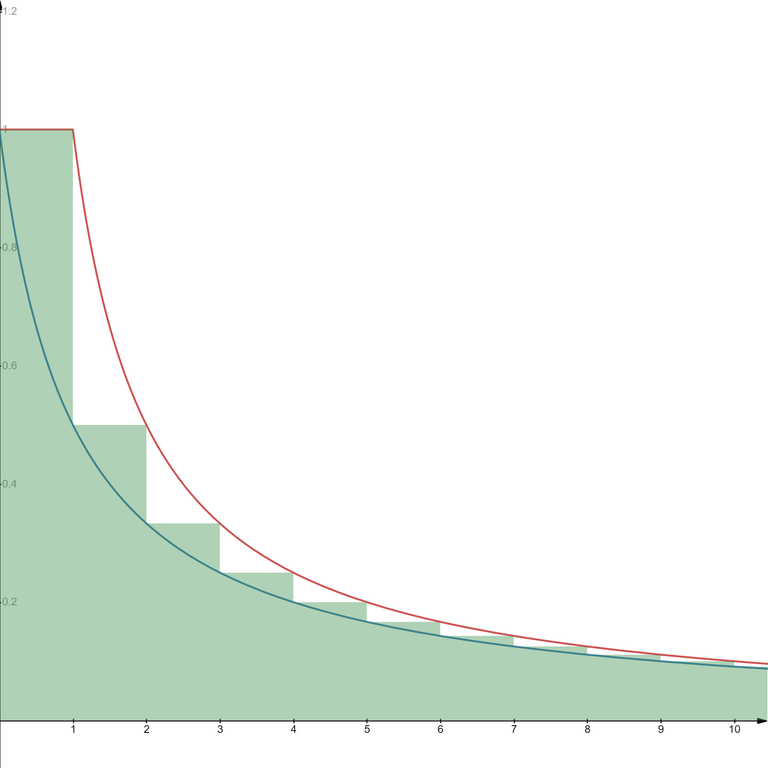
On the image, the area under the red curve (the function $$$f(x) = \min\left(1, \frac1x\right)$$$) entirely covers the bar chart, so we must have
$$$\displaystyle H_n \le \int_0^n f(x) \, \mathrm{d} x = 1 + \int_1^n \frac1x \, \mathrm{d} x = 1 + \ln n.$$$On the other hand, the bar chart completely covers the area under the blue curve (the function $$$g(x) = \frac1{x + 1}$$$), so we must have
$$$\displaystyle H_n \ge \int_0^n g(x) \, \mathrm{d} x = \int_0^n \frac1{x + 1} \mathrm{d} x = \ln (n + 1).$$$In total
$$$\ln (x + 1) \le H_n \le 1 + \ln n,$$$so indeed $$$H_n = \Theta(\log n)$$$.
This fact is useful in calculating complexities of certain algorithms. In particular, this is common in algorithms that look like this:
1 for i in 1..n:
2     for (int k = i; k <= n; k += i):
3         # whatever
For a fixed $$$i$$$, no more than $$$\frac{n}{i}$$$ values of $$$k$$$ will be visited, so the total number of hits to line 3 will be no more than
$$$ \frac{n}{1} + \frac{n}{2} + \cdots + \frac{n}{n} = n H_n,$$$so the complexity of this part of the algorithm is $$$O(n \log n)$$$.
Worked example: Divan and KostomukshaThis problem is from Codeforces round #757. Link to the problem: 1614D1 - Divan and Kostomuksha (easy version), we are only solving the easy version here.
Given an array $$$A$$$ consisting of positive integers, you want to reorder its elements such that the following value is maximized:
$$$ \displaystyle \sum_{i = 1}^n \gcd(A[1], \ldots, A[i]). $$$Lets think about the sequence formed by $$$\gcd(A[1], \ldots, A[i])$$$. It is a decreasing sequence of numbers, with each element being a divisor of the previous one. Define $$$\mathrm{dp}[k]$$$ as the maximum sum of a prefix whose gcd is $$$k$$$. To calculate it, we should start the prefix with the optimal prefix for some multiple of $$$k$$$ and then add append all remaining elements that are multiples of $$$k$$$. We are left with an algorithm that looks roughly like this:
1 for k in 1..MAX_A:
2     # cnt_multiples[k] is the number of multiples of k in the array
3     # it is possible that there is no larger multiple of k to be the previous gcd
4     dp[k] = k * cnt_multiples[k]
5     for (j = 2 * k; j <= MAX_A; j += k):
6         # we subtract k * cnt_multiples[j] because these elements already have larger
7         # contribution to the gcd sum.
8         dp[k] = max(dp[k], dp[j] + k * cnt_multiples[k] - k * cnt_multiples[j])
The algorithm has exactly the form as seen above, thus its complexity is $$$O(C \log C)$$$, where $$$C$$$ is the maximum value in the array $$$A$$$.
7. $$$O(n^2)$$$ complexity of certain tree DPs
Suppose you are solving a tree problem with dynamic programming. Your DP states look like this: for every vertex $$$u$$$ you have a vector $$$dp[u]$$$ and the length of this vector is at most the number of descendants of $$$u$$$. The DP is calculated like this:
 1 function calc_dp (u):
 2     for each child v of u:
 3         calc_dp(v)
 4     for each child v of u:
 5         for each child w of u other than v:
 6             for i in 0..length(dp[v])-1:
 7                 for j in in 0..length(dp[w])-1:
 8                     # calculate something
 9                     # typically based on dp[v][i] and dp[w][j]
10                     # commonly assign to dp[u][i + j]
11
12 calc_dp(root)
The complexity of this is $$$O(n^2)$$$ (this is not obvious: when I first saw it I didn't realize it was better than cubic).
Boring proofBy induction. Let $$$u$$$ be a vertex with $$$m_u$$$ descendants. Let $$$v_1, \ldots, v_k$$$ be the children of $$$u$$$, with $$$m_{v_1}, \ldots, m_{v_k}$$$ descendants respectively. Assume that for each $$$i$$$, in a call to calc_dp(v_i) there are no more than $$$m_{v_i}^2$$$ hits to line 8 (including the recursive hits). We will prove that if calc_dp(u) is called, line 8 will be hit no more than $$$m_u^2$$$ times.
The number of times line 8 will be hit is no more than
$$$\displaystyle \sum_{i} m_{v_i}^2 + \sum_i \sum_{j \ne i} m_{v_i} m_{v_j}.$$$The first sum comes from the recursive calls (by the induction hypothesis), the second is just directly translated from lines 4 to 7. Now notice that
$$$ \begin{align*} \displaystyle \sum_{i} m_{v_i}^2 + \sum_i \sum_{j \ne i} m_{v_i} m_{v_j} &= \sum_{i} m_{v_i}^2 + \sum_i \sum_j m_{v_i} m_{v_j} - \sum_{i} m_{v_i}^2 = \\ &= \left( \sum_i m_{v_i} \right)^2 \le \left( 1 + \sum_i m_{v_i} \right)^2 = m_u^2. \end{align*} $$$We now apply this result to the root, which of course has $$$n$$$ descendants, therefore the total complexity comes to $$$O(n^2)$$$.
Visual proofConsider the algorithm for a fixed $$$u$$$. For each child $$$v$$$ of $$$u$$$, we associate every position in the array $$$\mathrm{dp}[v]$$$ with a descendant of $$$v$$$. The array $$$\mathrm{dp}[v]$$$ is no longer than the number of descendants of $$$v$$$, so we can make sure no two elements in the subtree are associated with the same elements in the array.
Now, we iterate over all pairs $$$\left< v, i \right>$$$ and $$$\left< w, j \right>$$$, where $$$v$$$ and $$$w$$$ are different children of $$$u$$$. Instead of iterating over all pairs, let's think about iterating over the corresponding vertices $$$a$$$ and $$$b$$$. For a fixed $$$u$$$, we never visit the same pair of vertices twice. But in fact, the lowest common ancestor of $$$a$$$ and $$$b$$$ must be $$$u$$$, because $$$v$$$ and $$$w$$$ are different children of $$$u$$$. So in fact, we never visit the same pair of vertices during the course of the whole algorithm!
The number of times line 8 is hit must therefore be no larger than the number of different pairs of vertices in the tree, which is of course $$$O(n^2)$$$.
Worked example: Miss PunyverseThis problem is from ICPC Manila 2019 and also Codeforces round #607. Link to the problem: 1280D - Miss Punyverse.
You are given a tree on $$$n$$$ nodes; every node has an integer written on it. You want to partition the tree into $$$m$$$ connected regions such that the number of regions with a positive sum is maximized. $$$m \le n \le 3000$$$.
For any $$$u$$$, let $$$\mathrm{dp}[u][k]$$$ be the maximum pair $$$\left< t, s \right>$$$, such that
- the subtree of $$$u$$$ is partitioned into $$$k$$$ regions;
- the number of positive regions among them is $$$t$$$;
- the sum of the region $$$u$$$ is located in — the one we can possibly enlarge — is $$$s$$$.
An exercise to the reader: why is it sufficient to consider the maximum pair $$$\left< t, s \right>$$$?
The transitions to this DP can be calculated in a way similar as discussed above. For a given $$$u$$$, we start "building" the array $$$\mathrm{dp}[u]$$$ by iteratively considering new children of $$$u$$$ and "merging" them into the array $$$\mathrm{dp}[u]$$$. For each child $$$v$$$, we consider all pairs $$$\mathrm{dp}[u][i]$$$ and $$$\mathrm{dp}[v][j]$$$, and we put the calculated result into $$$\mathrm{dp}[u][i + j]$$$. With ideas similar as above, we can show that this has the complexity $$$O(n^2)$$$ as well.
8. Probabilistic treatment of number theoretic objects
This trick is not mathematically rigorous. Still, it is useful and somewhat reliable for use in heuristic/"proof by AC” algorithms. The idea is to pretend that things in number theory are just random. Examples:
- Pretend the prime numbers are a random subset of the natural numbers, where a number $$$n \ge 2$$$ is prime with probability $$$\frac1{\log n}$$$.
- Let $$$p > 2$$$ be prime. Pretend that the quadratic residues modulo $$$p$$$ are a random subset of $$$1, \ldots, p-1$$$, where a number is a quadratic residue with probability $$$\frac12$$$.
A quadratic residue modulo $$$p$$$ is any number $$$a$$$ that can be represented as a square modulo $$$p$$$; that is, there exists some $$$b$$$ such that $$$a \equiv b^2 \pmod{p}$$$.
The actual, mathematically true facts:
- There are $$$\Theta \left( \frac{n}{\log n} \right)$$$ primes up to $$$n$$$.
- Given a prime $$$p > 2$$$, there are exactly $$$\frac{p - 1}{2}$$$ quadratic residues.
Worked example: Elly's Different PrimesThis problem is from Topcoder Open 2020 Round 1B. Link to the problem. I chose an example from Topcoder because it is very common to see this idea there.
A prime is called different if all of its digits are different. Given an integer $$$n$$$, find the different prime closest to $$$n$$$. We have $$$1 \le n \le 5 \cdot 10^7$$$.
The solution is to simply iterate over numbers slightly below and above $$$n$$$ and check if they are prime. There is really no need to do anything cleverer here. Prime numbers are plentiful, so you will reach your target very quickly: it is probably even fast enough to check whether a number is prime completely naively by trial division.
Worked example: Number TheoryThis problem is from Moscow Workshops Discover Riga/Singapore 2019, 300iq contest. I don't know if you can submit it anywhere.
Given a prime $$$p$$$. For any $$$x$$$, we can decompose it as follows: $$$x \equiv a^2 + b^2 \pmod{p}$$$ for some $$$a, b$$$. This is always possible, but we are interested in the "best" way — the one with the smallest $$$a$$$. Let $$$f(x)$$$ be the smallest $$$a$$$ such that this is possible. You want to find the maximum of $$$f(0), f(1), \ldots, f(p - 1)$$$. $$$p \le 10^5$$$.
Consider a fixed $$$x$$$. How to check if a particular $$$a$$$ is suitable? A simple rearrangement gives $$$x - a^2 \equiv b^2 \pmod{p}$$$, so all we need to do is check if $$$x - a^2$$$ is a quadratic residue. This can be done by precomputing all quadratic residues modulo $$$p$$$.
The completely naive solution then would be to iterate over all $$$a$$$, starting from 0, and stopping once we find an $$$a$$$ such that $$$x - a^2$$$ is a quadratic residue. And that turns out to be good enough because at every step we have $$$\frac{1}{2}$$$ probability of encountering a quadratic residue. Repeat this for each $$$x$$$ and you have an unproven expected $$$O(n)$$$ complexity.
Many actual, practical number theoretic algorithms use these ideas. For example, Pollard's rho algorithm works by pretending that a certain sequence $$$x_i \equiv x^2_{i - 1} + 1 \pmod{n}$$$ is a sequence of random numbers. Even the famous Goldbach's conjecture can be seen as a variation of this trick. On a lighter note, this is also why it is possible to find prime numbers like this:
A prime number1111111111111111111111111111111111111111111111111111111111
1111111111111111111111111111111111111111111111111111111111
1111888888888888881111888888888888881111888888888888881111
1111888888888888881111888888888888881111888888888888881111
1111888811111111111111888811111111111111111118888111111111
1111888811111111111111888811111111111111111118888111111111
1111888888888881111111888888888881111111111118888111111111
1111888888888881111111888888888881111111111118888111111111
1111888811111111111111888811111111111111111118888111111111
1111888811111111111111888811111111111111111118888111111111
1111888811111111211111888811111111111111111118888111111111
1111888811111111111111888811111111111111111118888111111111
1111111111111111111111111111111111111111111111111111111111
1111111111111111111111111111111111111111111111111111111111
Prime numbers are plentiful, so it's easy to create such pictures by taking a base picture and changing positions randomly.
9. LCAs induced by a subset of vertices
Given a tree and a subset of vertices $$$v_1, v_2, \ldots, v_m$$$. Let's reorder them in the (preorder) DFS order. For any $$$i$$$ and $$$j$$$ with $$$v_i \ne v_j$$$, $$$\mathrm{lca}(v_i, v_j) = \mathrm{lca}(v_k, v_{k + 1})$$$ for some $$$k$$$. In other words: the lowest common ancestor of any two vertices in the array can be represented as the lowest common ancestor of two adjacent vertices.
ProofPick some $$$v_i$$$ and $$$v_j$$$ and assume $$$i < j$$$. Let $$$\mathrm{lca}(v_i, v_j) = u$$$. If $$$u = v_i$$$, then we can use $$$v_i$$$ and the first descendant of $$$v_i$$$ that appears in the subset; they must be adjacent. Otherwise, let $$$w$$$ be the child of $$$u$$$ whose subtree contains $$$v_i$$$. Because the vertices are in the DFS order, the vertices in the subtree of $$$u$$$ must form a contiguous range among $$$v_1, \ldots, v_m$$$. Similarly, the vertices in the subtree of $$$w$$$ must form a contiguous range, contained in the range for $$$u$$$. We can use the last vertex in the subtree of $$$w$$$ and the first vertex in the $$$u$$$-range that is not contained in $$$w$$$. Neither of them is an empty set, because they contain $$$v_i$$$ and $$$v_j$$$ respectively.
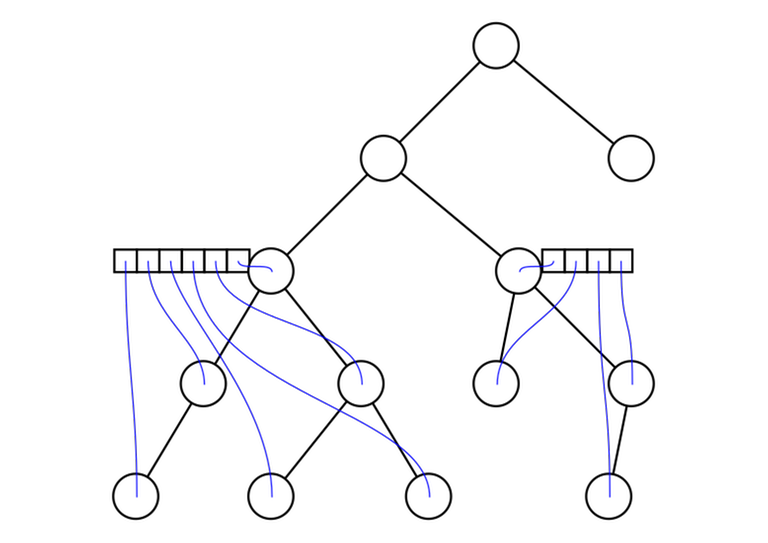
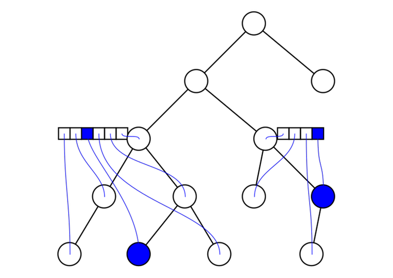
An application: virtual treesThis fact is useful for calculating the so-called "virtual trees". In some problem, such as 613D - Kingdom and its Cities, you are given many queries, each query consists of a subset of vertices. To answer these queries, it is not necessary to consider the whole tree. It is sufficient to consider the given subset of vertices, as well as some additional vertices where paths from the given vertices to one another "join up". They form a smaller tree with much fewer vertices, called the virtual tree:
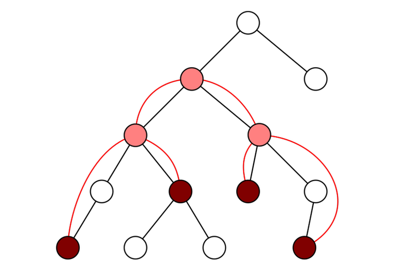
In this picture, the given subset of vertices is in dark red. To join them up while preserving the structure (it's hard to formally explain what the actual requirement is, but hopefully the idea is clear) we need to add the pink vertices. The dark red and pink vertices together form the vertices of the virtual tree. The edges of the virtual tree are shown in red.
Notice that the vertices making up the virtual tree are exactly those of the form $$$\mathrm{lca}(u, v)$$$, where $$$u$$$ and $$$v$$$ are part of the given subset of vertices. Using the fact that we just learned, we can find the vertices that form the virtual tree by sorting the given subset by DFS order, taking the LCAs of all adjacent pairs of vertices, and removing the duplicates. To find the edges of the virtual tree, you can again sort all the vertices of the virtual tree, and use a stack-like idea to connect them up.
10. Erdős–Szekeres theorem
Consider a permutation $$$p$$$ with length $$$n$$$. At least one of the following is true:
- There exists an increasing subsequence with length $$$\sqrt{n}$$$.
- There exists a decreasing subsequence with length $$$\sqrt{n}$$$.
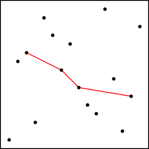
On this image we can see one possible decreasing subsequence of length 4 in a permutation of length 16. There are many options, some longer than 4.
Alternatively, we may phrase this as a fact about the longest increasing and decreasing sequences.
ProofIt can be proven directly, but I like to think of it as a special case of Dilworth's theorem.
To formulate it as a case of Dilworth's theorem, we define a partial order: $$$i \preceq j$$$ if and only if $$$i \le j$$$ and $$$p_i \le p_j$$$. An "antichain" is then a decreasing subsequence. A "chain" is an increasing subsequence. Dilworth's theorem states:
Consider splitting the permutation into increasing subsequences. The length of the longest decreasing subsequence is exactly the minimum number of increasing subsequences needed.
Suppose that the length of the longest decreasing subsequence $$$\ell$$$ and $$$\ell < \sqrt{n}$$$. Then we can split the permutation into $$$\ell$$$ increasing subsequences; as the sum of their lengths is $$$n$$$, at least one of them will be at least $$$\sqrt{n}$$$.
This proves that if the longest decreasing subsequence is shorter than $$$\sqrt{n}$$$, then there exists an increasing subsequence with length at least $$$\sqrt{n}$$$. A similar argument shows that if the longest increasing subsequence is shorter than $$$\sqrt{n}$$$, then there exists a decreasing subsequence with length at least $$$\sqrt{n}$$$.
Worked example: ParadeThis problem is from Algorithmic Engagements. I know this problem from "best problem in 2019" discussion, I'd be grateful if someone sent a link.
Given $$$n = 3 \cdot 10^5$$$ points on a plane, you get to pick a subset of 500 points and need to solve the Traveling Salesman problem on the chosen subset.
You can use a variant of this idea: we can either find a path with length at least $$$\sqrt{n}$$$, where $$$x$$$ and $$$y$$$ are both increasing; or a path with length at least $$$\sqrt{n}$$$, where $$$x$$$ is increasing and $$$y$$$ is decreasing. Solving the Traveling Salesman problem on such subsets is trivial. $$$500 \le \sqrt{n}$$$, so no worries there.
Thank you for reading! 10 is a good number, I think I've reached a good length of a blog post for now.


